Seismic sections are usually subjected to some processing sequence for noise reduction. If the noise has appreciable energy outside the frequency range of the useful signal, these sequences are effective and if accurate NMO and STATIC are done, data cluster after stack can be greatly reduced. Spectrum of noise however do overlaps the signal spectrum and 100% noise removal is difficult and because interference affects the seismic response of acquisition system for closely spaced boundaries, these lead to data cluster and biased seismic section prior to migration.

In this paper, a simple algorithm for enhancing the resolution of high frequency seismic data was developed, a two-step method which utilizes data transformation by root-mean-square deviation (RMSD). 

It was demonstrated how this algorithm could be used for noise reduction in image reconstruction and still retain the amplitude spectrum as the original section. It was successfully applied to real data.

 INTRODUCTION

The seismic reflection method of exploration is used to map the configuration and nature of remote and inaccessible rock layers beneath the subsurface of the earth (Silvia and Robinson, 1979).

Seismic traces that record the earth responses will be polluted by noise and distortion, thus losing continuity of some of the seismic pattern (Sheriff, 1972). For seismic reflection interpretation, the data processing routines must separate signals from noise and processing routines are linked together by a need to make the seismic data sensible (shon and Yamamoto, 1992). Data processing objectives are to improve data quality and present them in a convenient form. If the noise has appreciable energy outside the principal frequency range of the signal, frequency filtering can be used to advantage of reducing noise.

However, the spectrum of noise often overlaps the signal spectrum and then frequency filtering is of limited value in improving record quality (Telford etal). Stacking of NMO and DMO corrected seismogram amongst its objectives aims at increasing signal to noise ratio, that is, enhance reflection events relatively and suppress unwanted signal after stack.

In practice, the events which are not of reflection types have not been completely removed due to try and error choice of moveouts velocities and linear interpolation scheme for velocity smoothing between CDPs considered for velocity analysis, this tend to produce data cluster and unsatisfactory quality stack, in most cases gives a biased seismic section prior to migration. Even though, appropriate choice of filter’s parameters for a suitable filter can help in reducing this problem, in some processing environment, exhaustion of production library can witness occasion where proper filter’s algorithm is not available for the choice of required and accessible parameters.

The seismic acquisition system detects only a limited proportion of geological boundaries and when these boundaries are closely spaced, interference is known to affect the seismic response, complicating or making impossible our perception of the geology. For these complex natures of processing sequences, practical processing therefore requires a number of steps which are subjective in nature and it becomes necessary to facilitate, during processing, easy recognition of the individual reflection because of the significance of each and of them to each other in geological interpretation of seismic sections.

Root-mean-square deviation has been used in diverse area of physical and social sciences: in meteorology to see how effectively a mathematical model predicts the behaviour of the atmosphere; in economics, it is used to determine whether an economic model fits economic indicators; in hydrogeology, RMSD and NRMSD are used to evaluate the calibration of a groundwater model; in computational neuroscience, the RMSD is used to assess how well a system learns a given model; and in imaging science, RMSD is part of the peak signal-to-noise ratio, a measure used to assess how well a method to reconstruct an image performs relative to the original image; to mention but few.

In this paper a two-step method for removing data cluster and hence improving the resolution of high frequency data prior to migration, which utilises maximum root-mean-square-deviation (RMSD) is presented.

                                                            THE ALGORITHM

Let ξjt be the seismic wavefields contributing to the data population for a seismic trace, where,

Normal 0 false false false EN-US X-NONE X-NONE

/* Style Definitions */ table.MsoNormalTable {mso-style-name:"Table Normal"; mso-tstyle-rowband-size:0; mso-tstyle-colband-size:0; mso-style-noshow:yes; mso-style-priority:99; mso-style-qformat:yes; mso-style-parent:""; mso-padding-alt:0in 5.4pt 0in 5.4pt; mso-para-margin:0in; mso-para-margin-bottom:.0001pt; mso-pagination:widow-orphan; text-autospace:ideograph-other; font-size:10.0pt; font-family:"Calibri","sans-serif";}

/* Style Definitions */ table.MsoNormalTable {mso-style-name:"Table Normal"; mso-tstyle-rowband-size:0; mso-tstyle-colband-size:0; mso-style-noshow:yes; mso-style-priority:99; mso-style-qformat:yes; mso-style-parent:""; mso-padding-alt:0in 5.4pt 0in 5.4pt; mso-para-margin:0in; mso-para-margin-bottom:.0001pt; mso-pagination:widow-orphan; text-autospace:ideograph-other; font-size:10.0pt; font-family:"Calibri","sans-serif";} U_it is the corrected surface measured wavefields and ξ_jt is the algebraic sum of such corrected surface measured wavefield contributed to by traces from the same common mid-point (CMP) gather, and t is the time.

Normal 0 false false false EN-US X-NONE X-NONE

/* Style Definitions */ table.MsoNormalTable {mso-style-name:"Table Normal"; mso-tstyle-rowband-size:0; mso-tstyle-colband-size:0; mso-style-noshow:yes; mso-style-priority:99; mso-style-qformat:yes; mso-style-parent:""; mso-padding-alt:0in 5.4pt 0in 5.4pt; mso-para-margin:0in; mso-para-margin-bottom:.0001pt; mso-pagination:widow-orphan; text-autospace:ideograph-other; font-size:11.0pt; font-family:"Calibri","sans-serif"; mso-ascii-font-family:Calibri; mso-ascii-theme-font:minor-latin; mso-fareast-font-family:"Times New Roman"; mso-fareast-theme-font:minor-fareast; mso-hansi-font-family:Calibri; mso-hansi-theme-font:minor-latin; mso-bidi-font-family:"Times New Roman"; mso-bidi-theme-font:minor-bidi;}

ξ_jt can be nagative, zero ore positive depending on the relative magnitude of the time-coincident values U_it, with i = 1, 2, 3, 4, ............, k and k is the fold of stack. Provided the static and dynamic corrections are accurately made, signal-to-noise improvements for random noise should be about 2.5 for k = 6 and about 5 for k = 24 (Telford etal).

Structural and stratigraphic processing combined, require that at least one ξ exists between two values which contribute to the image of two adjacent reflecting interfaces constituting a bed such that v\:* {behavior:url(#default#VML);} o\:* {behavior:url(#default#VML);} w\:* {behavior:url(#default#VML);} .shape {behavior:url(#default#VML);}

Normal 0 false false false EN-US X-NONE X-NONE /* Style Definitions */ table.MsoNormalTable {mso-style-name:"Table Normal"; mso-tstyle-rowband-size:0; mso-tstyle-colband-size:0; mso-style-noshow:yes; mso-style-priority:99; mso-style-qformat:yes; mso-style-parent:""; mso-padding-alt:0in 5.4pt 0in 5.4pt; mso-para-margin:0in; mso-para-margin-bottom:.0001pt; mso-pagination:widow-orphan; text-autospace:ideograph-other; font-size:10.0pt; font-family:"Calibri","sans-serif";}

ξ_{jt > 0}

for Normal 0 false false false EN-US X-NONE X-NONE

ξ_j-n,t-t’ > 0 and ξ_j+n,t+t’ > 0, ξ ϵ R

Where t’ = n∆t, n ≥ 1 and ∆t is the sampling or re-sampling interval, t is the instantaneous time and t’ is an arbitrary time interval. In practice, imperfect and/or limitation of efficiency of acquisition system has yielded a stacked seismic section which contains one or more unresolved thin bed as a result of the existence of inequalities

 ξ_{jt > 0 for all} ξ ϵ R

Where R defines the ensemble of data within the time gate (t – t’)–(t + t’).

Inequalities (3) and (4) may lead to false stratigraphic and structural interpretation and meaningless section.

Seismic data recording can be carried out for any length of time; therefore this is viewed as of infinite population. Instead of working with this population, a representative member is chosen, i.e, all Normal 0 false false false EN-US X-NONE X-NONE MicrosoftInternetExplorer4

/* Style Definitions */ table.MsoNormalTable {mso-style-name:"Table Normal"; mso-tstyle-rowband-size:0; mso-tstyle-colband-size:0; mso-style-noshow:yes; mso-style-priority:99; mso-style-qformat:yes; mso-style-parent:""; mso-padding-alt:0in 5.4pt 0in 5.4pt; mso-para-margin:0in; mso-para-margin-bottom:.0001pt; mso-pagination:widow-orphan; font-size:11.0pt; font-family:"Calibri","sans-serif"; mso-ascii-font-family:Calibri; mso-ascii-theme-font:minor-latin; mso-fareast-font-family:"Times New Roman"; mso-fareast-theme-font:minor-fareast; mso-hansi-font-family:Calibri; mso-hansi-theme-font:minor-latin; mso-bidi-font-family:"Times New Roman"; mso-bidi-theme-font:minor-bidi;} ξ ≥ 0 and neglect all ξ < 0 for the time being. Since the choice here is subjective, the chosen sample is considered as a biased sample.

 

Let r be the length of the data in a trace, i.e, the trace length and let the size of all ξ ≥ 0 be l and those of ξ < 0 be m, then it follows that

 

The sample mean is therefore given by 

For a sample of with mean x, where the observation is x_i, the variance is defined as,

Sample variance,

 

Where N is the sample size and the sample standard error, is defined as,

 

The above equations for sample variance and standard error hold for unbiased sample. For biased sample, N-1 IS replaced by N(O.O Ayeni) and the standard deviation becomes

 

Equation (8) is the generalized expression for root-mean-square deviation. Since we are dealing with biased sample in this paper,the above equation is employed.

Therefore with  ,  and N = n = l, the expression for root-mean-square deviation as applied to this work becomes

 

Let

 ,  where j = 1, 2, 3, .........., r-m, and k = 1, 2, 3, ........,  

 is the objective function. Assuming there are Common Mid Points (CMPs) in a stacked section, it is desired to find s for individual trace in a stacked seismic section such that is maximum. Let this maximum value be . High frequency seismic data resolution by data transformation by root mean square deviation requires the operation

 

 

APPLICATION IN IMAGING SCIENCE:

 

(a)   APPLICATION IN SEISMIC IMAGE RECONSTRUCTION

Seismic data which is available only as film or paper can be an underutilized resource of the exploration department most especially if these sections are unmigrated. Where archive copies of the processed stacked or migrated tapes are not available, seismic image reconstruction techniques have been able to reproduce digital traces in SEG-Y format directly from the available plots.

This does not only allow modern processing and display techniques to be used to enhance the original data, but also permits data loading to interpretation workstation.

Seismic sections on paper on films are scanned using high resolution seismic document scanner. Old sections and dirty originals are cleaned up at the input to reconstruction algorithm stage using dynamic contrast setting and raster editing prior to creating raster file.

However 100% successful contrast setting can only be achieved if there is sufficient threshold differential between the cut off threshold of the background and that of the positive variable regions where troughs and peaks exist for the seismic traces. Practice has however experienced occasions whereby there no contrast between the two cut-off thresholds, case for which low scanning threshold leads to loss of high frequency events and so one is forced to scan at threshold which will resolve the high frequency events but with the reconstruction algorithm vectorizing some portions of the background as positive variable area.

However, after a series of fine-tuning, the desired result can be achieved. Considering contractual time, this may not be favorable.

Let the vectorised waveform after trace reconstruction be defined by the function

 

A is a time dependent amplitude and t is the instantaneous time.

To ensure that the frequency contents of the data are preserved on application of the algorithm developed here, we must have the following conditions met before the data transformation:

 

 

APPLICATION AS A POST-STACK DATA FILTER

 

The equation of standard deviation as applied to seismic trace for noise reduction is given by (Shon and Yamamoto, 1992), with the mean of the data in a trace taken to be zero, as

 

 

 

Where $x_i$ is the $i^{th}$ data; N is a trace length and $\sigma_u$ is the standard deviation. In their algorithm, the whole data length is considered and consequently the unbiased variance, $\sigma_u^2$.

 

 

 

The threshold specified by equation (9) can be shown to have advantage over the one specified by (10) in retaining data level, aprt from the fact that here, data is not deleted but transformed, in the sense of amplitude spectrum preservation thus;

 

If the positive wavefields and the negative wavefields are specified by x_j and x_k respectively, then equation (10) can be written, with x = x and N = t, as

 

 

R is as previously defined.

 

 

The mean value of the seismic trace is nearly zero over a whole trace (Shon, 1990), or assuming a harmonic or Gaussian trace, it suffices to write

 

 

 

PROCEDURE FOR THE APPLICATION OF THE ALGORITHM TO DATA SAMPLE

 

The standard deviation of the data for each trace is determined in the seismic section.

To ensure that conditions specified in (9b) are met for operation in (9a) to follow, a time gate defined by

is chosen such that the gate length is n∆t, ∆t being the sampling or re-sampling interval and the window is successfully slides down each of the trace length separately. The overlap in the sliding window must be (n – 1)∆t.

 

  

 

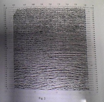
Figure 2 shows data from offshore Nigeria. The section was subjected to single trace test (STT) of the algorithm. The trace coincides with Common Depth Point (CDP) 71 of the same figure. In this test, the time gate is chosen such that the gate length is 12ms and the overlap in the sliding window is 8ms with the sampling interval of 4ms.

 

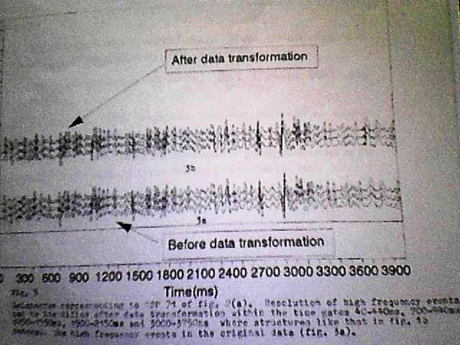
Figure 3a is the trace, repeated, before data transformation; while figure 3b is the same trace, repeated, after transformation.

REFERENCES:

Ayeni,O.O,1981 Statistical adjustment and analysis of data (with application in Geodetic Surveying and Photogrammetry), University of Lagos Press

Marsden, D. 1993 ,Static  corrections - A review, Parts I, II, III; The leading edge, Vol. 12 No 1-3

Shon, H and Yamamoto, T, 1992, Simple data processing procedure for seismic section noise reduction, Geophysics, Vol. 37, 1084-1087

Silvia, M.T and Robinson, E.A, 1979, Deconvolution of geophysical series in the exploration for oil and natural gas: Elsevier Science Publication Co. Inc

Telford W.M, Geldart D.P, Sheriff R.E, Keys D.A, 1976, Applied Geophysics, Cambridge University Press.