

Now, the purpose of this article is multifold. First of all, I wish to publicize the slides (which you can freely access in three separate files: part 1, part 2, part 3), with the hope that some of you will actually read them (they should be beneficial to anybody with a PhD in particle physics who does not consider herself an expert in statistics, as well as to undergraduates and graduate students who have an interest in not remaining ignorant in these matters forever), possibly reporting any mistake or inconsistency. This is in the interest of improving the material for the next time I will be able to use it.
The second reason of mentioning my Statistics course here is shameless self-promotion. I had fun giving the course, and I would be happy to be given another chance - to improve one has to practice! So if you are a graduate student or a young postdoc and you think it would be nice if your University or institute would feature such a set of lectures, consider suggesting your advisor to organize them! I think there is too little awareness on the subtleties of the practice of statistics in data analysis for particle physics, and I would be happy to contribute to raising the education around.
Third, I want to make an example of the pitfalls you can avoid if you know statistics, by pasting here the result of a study of two test statistics used to fit a data histogram: Pearson's chisquare and Neyman's chisquare. Neyman's chisquare is the sum of the squared differences between the measured values and the fit function, divided by the individual measured variances, while Pearson's chisquare substitutes the denominator with the best-fit variance. It is important to note that both test statistics therefore estimate the variance of the true value to "normalize" the observed squared deviations between observations and model.
The fact that the variances at the denominator are estimates instead than the true values causes the minimization of the resulting chisquares to produce different results. Let us take a simple case of the fit to a constant of a 100-bin histogram, where each bin contains Poisson-distributed event counts. While the maximum likelihood estimate of the value of the constant is just the sum of the bin entries divided by the number of bins (the arithmetic average!), the Pearsons and Neyman chisquares, if minimized, produce biased estimates of the constant.
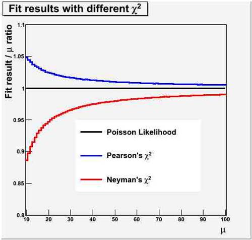 The figure on the right show the amount by which the two chisquare fits (Pearsons, in blue, and Neyman, in red) under- or overestimate the true value of the constant (in black - which coincides with the maximum likelihood estimate). On the horizontal axis is the real value of the Poisson mean from which 100 bins were populated; on the vertical axis is the fractional bias on the fit result.
To understand the reason why the two test statistics are biased (but note, they are asymptotically unbiased in the large-sample limit) we need to put ourselves in the pants of the minimization routine.
What we are doing when we fit a constant through a set of 100 bin contents is to extract the common, unknown, true value μ from which the entries were generated, by combining the 100 measurements, each of which is a Poisson estimate of this true value. Each should have the same weight in the combination, because each is drawn from a Poisson of mean μ, whose true variance is also equal to μ (a property of the Poisson distribution!). But, having no μ to start with, we must use estimates of the variance as a (inverse) weight. So Neyman's chisquare gives the different observations different weights 1/N, where N is the bin content. Since negative fluctuations (N < μ) have larger weights, the result is downward biased!
What Pearsons' chisquare does is different: it uses a common weight for all measurements, but this is of course also an estimate of the true variance V = μ : the denominator of Pearsons' chisquare is the fit result for the average, call it μ*. Since we minimize that chisquare to find μ*, larger denominators get preferred, and we get a positive bias: μ* > μ!
The bottomline is the following: when possible, especially when statistics is poor, use a likelihood to fit your data points !


Comments