

In data analysis, Gaussian distributions are ubiquitous. But that does not mean they are the only distribution one encounters ! In fact, it is unfortunately all too common to find unmotivated Gaussian assumptions in the probability density function from which the data are drawn. Usually one makes such assumptions implicitly, and so these remain hidden between the lines; the result is almost never dramatic, and those few among us who believe that doing science requires rigor are the only ones who are left complaining.
These days I happen to be putting together a course of basic Statistics for HEP experimentalists, which I will be giving in the nice setting of Engelberg (Switzerland) later this month. Since I want to give a HEP example of the pitfall of the Gaussian assumption, which one needs to avoid in data analysis by having always clear in mind the question "What is the pdf from which I am drawing my data ?", I dusted off one complaint I had with the Opera measurement of neutrino velocities -the reloaded analysis, published one month ago here.
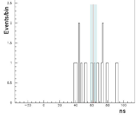 Opera collected 20 good neutrino interactions from narrow-bunched proton spills at CNGS at the end of October. These 20 events are a golden set because in practice every single one of them is sufficient to measure the time spent by neutrinos to travel from CERN to Gran Sasso: one needs not mess with the proton bunch time profile anymore, since the latter is a 3ns-wide spike in this case. You can see the 20 timing measurements in the histogram on the right.
Unfortunately, it transpires that the Opera time measurement is subjected to a +-25 ns jitter, which means that they only have 50 nanosecond accuracy on their delta-t measurements. In other words, their measured times are all displaced by a random amount within a box of 50 nanoseconds width. Those 20 events are therefore sampled from a uniform distribution, and all that is left to measure, in order to find the best estimate of the travel time, is the center of that distribution.
But here comes in the implicit Gaussian assumption: Opera proceeds to take the sample mean (the arithmetic linear average, <t>=1/N Sum_i t_i) of the 20 timing measurements t_i in order to estimate the center of the 50ns box.
At this point, you could well be a little puzzled, asking yourself what the hell I am talking about: surely, the sample mean is a good way to estimate the location of a distribution, even if non Gaussian, right ?
Wrong. The sample mean is a very stupid thing to use for a box distribution. The reason is best understood by considering the following alternative procedure: order your data {t_i} from the smallest to the biggest, and take the smallest measurement t_min and the biggest t_max; throw away all the others (18 precious neutrino interactions are thus flushed in the toilet! Can you hear them scream ?). The location estimator which happens to be the uniformly minimum variance unbiased one, in this case, is t_mid = (t_max+t_min)/2.
What happens is that since all the t_i are sampled from a uniform distribution, the information that each of the 18 remaining events carry for the location of the box, once you have picked the minimum and the maximum, is null! They carry no information whatsoever, because each of these additional timing measurements, painfully obtained by Opera, equates to shooting at random a number within the bounds [t_min,t_max] ! Pure noise !
In practical terms, the sample mean is NOT the minimum variance estimator: the sample mean <t> is affected by the noise that is instead discarded by the sample midrange t_mid. The sample midrange is the UMVU (uniformly minimum variance unbiased) estimator, not the sample mean! A few lines of code allow us to estimate the expected value of the uncertainties in the two estimators: we get that the expected statistical error on the sample mean of 20 values drawn from a box distribution of 50ns width is 3.3 ns, while the expected statistical error on the sample midrange is 1.66 ns.
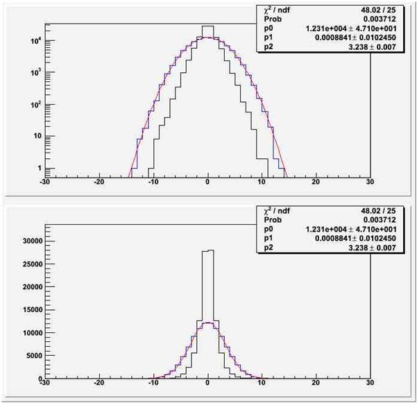
Below you can see the distribution of the two estimators <t> and t_mid for 100,000 repeated experiments where 20 timings are drawn at random from a box having range [-25,+25]. On the top the two are plotted in a semi-logarithmic graph, and on the bottom they are shown on a linear scale. You can clearly see that the black histogram (representing t_mid) is twice as narrow as the blue one (representing <t>). In case you ask, the former has a Laplace distribution (technically it is Nt which has a Laplace distribution, but that's a detail), while the latter is of course Gaussian.
Update: As mentioned at the top, I am leaving the "interim" conclusions live below, but I am further commenting at the end, revising them significantly.
In summary, not only did Opera quote a value, <t>=62.1 ns, which is not making the best use of their data; in so doing, they double the statistical uncertainty of their measurement! They quote <t>=62.1+-3.7 ns, while using the midrange they would have quoted instead t=65.2+-1.7 ns.
If this sounds irrelevant to you, consider that the CERN beam ran for a couple of weeks (from October 22nd to November 6th) to deliver those 20 interactions to Opera. They could have ran for just a week instead, when Opera could still obtain a 3ns-ish statistical uncertainty, had they used the right estimator.
Update: revised conclusions below.
As you can read in the comments thread, a reader points out that if each timing measurement suffers from a random Gaussian smearing, the conclusions can change on whether the UMVU estimator is still the sample midrange or rather the sample mean. Indeed, going back to my toy Monte Carlo, I find that if, in a 20-event experiment, each measurement is subjected to a Gaussian smearing of size larger than 6ns then the best estimator returns to be the sample mean. The reason is that the distribution of the data becomes a convolution of Gaussian and Uniform, and the events "within" the spanned range [t_min,t_max] return to contain useful information for the location of the distribution.
 On the right you can see the rms of the two estimators (in ns) as a function of the sigma of the Gaussian smearing (also in ns). The sample midrange is the UMVU for a box, but it is not a robust estimator!
I am unable to determine whether Opera's timing measurements are indeed subjected to that effect; from a reading of their paper I am inclined to believe they are. Therefore, they may in the end have done the right thing. Nevertheless, I believe the article above retains the didactic value it was meant to have. Maybe I should just point out that Gaussians are indeed ubiquitous!


Comments