


The mathematical formalism of quantum mechanics can be built up on the basis of the following rules. Suppose that you want to calculate the probability of a particular outcome of a measurement M2, given the outcome of am earlier measurement M1. Here is what you have to do:
- Choose any sequence of measurements that may be made in the meantime.
- Refer to the possible sequences of outcomes as alternatives. (It pays to remember that alternatives are defined as sequences of measurement outcomes.)
- Assign to each alternative a complex number and refer to it as its amplitude.
- Then —
(Rule B) If the intermediate measurements are not made (and if it is impossible to find out what their outcomes would have been if they had been made), first add the amplitudes of the alternatives and then square the magnitude of the result.

In the particular case of a 2-slit experiment with electrons, the initial measurement indicates that an electron has been launched by/at an electron gun G, while the final measurement indicates the position — along an axis across the screen — at which the electron is detected. (If we assume that G is the only source of free electrons, then the detection of an electron behind the slit plate also indicates the electron’s launch at G.) A single intermediate measurement, if made, indicates the slit through which the electron went. Thus there are two alternatives with respective amplitudes AL and AR. To calculate these amplitudes, we need to know three things:
- AL is the product of two complex numbers, known as propagators, for which we will use the symbols <D|L> and <L|G>, respectively. Thus AL = <D|L> <L|G>. Likewise AR = <D|R> <R|G>.
- The magnitude of the propagator <B|A> is inverse proportional to the distance d(AB) between A and B.
- The phase of <B|A> is proportional to d(AB).
We need to appreciate how preposterous this is from a classical point of view. Classically, the probability with which the particle arrives at D (given that it comes from L) depends on whence it arrives at L. The reason this is so is that, classically, the momentum with which the particle departs from L is the same as that with which it arrives at L. If we make the idealizing and simplifying assumption that all our position measurements are precise, then the uncertainty principle tells us that, quantum-mechanically, the momentum with which the particle departs from L is as fuzzy as it gets. Therefore the place whence the particle arrives at L has no effect on the probability with which it arrives at D. Hence item (1).
To account for item (2), we imagine a sphere of radius R centered at A. Let p(R) be the probability with which a particle launched at A is found by a detector monitoring a unit area of the surface S of this sphere. Since the particle proceeds from A in no particular direction, p(R) is constant across S. Because the area of S is proportional to R2, and because the total probability of detecting the particle anywhere on S equals unity, p(R) is inverse proportional to R2. Hence the corresponding amplitude is inverse proportional to R, and from this we gather that the magnitude of <B|A> is inverse proportional to the distance between A and B.
To account for item (3), we take note of the fact that space does not come with an in-built metric. How — by means of which physical objects — we measure distances, is up to us. The measuring rods we choose as the most convenient ultimately depend on such basic physical processes as the propagation of a free particle from A to B. It stands to reason that the most convenient metric results if the phase of <B|A> only depends on the distance between A and B, and if it is proportional to this distance. Hence item (3).
No we can go ahead and calculate.
Since the slits are equidistant from G, <L|G> and <R|G> are equal, so to plot pA(D) as a function of the position of D, we only need to evaluate

The correct proportionality factor can be recovered by requiring that the area under the plot be equal to unity. In the same way we find
 which works out at
where Δ is the difference between d(DR) and d(DL), and k is the proportionality factor between d(AB) and the phase of <B|A>. Plotting the two probability distributions is now a matter of elementary geometry and appropriate software.
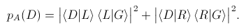
The probability of detection according to Rule A (the solid curve) is the sum of two probability distributions (the dotted curves), one for the electrons that went through L and one for the electrons that went through R:
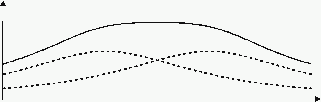
The probability of detection according to Rule B:
Let us now try to understand what happens under the conditions stipulated by Rule B.


Comments