

Heavy neutrinos N may explain the very small but finite mass of the three "regular" standard model (SM) neutrinos through a process called "see-saw", whereby the three neutrino masses are kept very small -much smaller than the mass of all other SM particles - by the large mass of N. The latter is inversely proportional to the former in this mechanism.
A heavy neutrino might be a very interesting body: a Majorana particle which is its own antiparticle. Two such things may then annichilate if they get in contact; furthermore, and more experimentally interesting, is the fact that processes involving Majorana neutrinos may violate lepton number conservation by two units.
Lepton number is something which in the SM is perfectly conserved: you can vary the number of electrons in a system only if you correspondingly vary the number of electron neutrinos by the opposite amount; and similarly -and independently- for muon and muon neutrinos, and for tau and tau neutrinos. In all processes involving these particles, it is like they "pass on" the "lepton flavour" as they interact. So, e.g., if a muon decays to a muon neutrino plus a W boson, then in so doing the muon yields the "muonness" to the muon neutrino. There is as a result one less muon in the system, but one more muon neutrino, and muon flavor has kept unvaried.
A Majorana neutrino N changes this scheme completely. Let us take a positively-charged W boson created in a proton-proton LHC collision, which -if N exists- may decay to a positive muon and a Majorana neutrino N: we write
 . A positive muon counts M=-1 for the muon flavour (it is the antiparticle of the negative muon which is taken as having M=1), so since the W has M=0, the produced N has M=+1 and all is well until now: both initial and final state have M=0 (M is an additive quantum number, so we just add +1-1=0 for the final state particles).
 Now, N can decide to decay as its own antiparticle, i.e. one of M=-1. So it may go
 . As a result of the production and decay process, we have a final state with two positive muons (the negative W can e.g. decay into a pair of jets). As a result of the existence of a particle carrying lepton number which is its own antiparticle, we have created two negative units of muonness out of nothing!
From an experimental point of view, such a Majorana particle is not too hard to find if it exists, as the production of final states with two positive muons in proton-proton collisions is very rare. All SM processes of this kind also yield an equal number of muon neutrinos, thus keeping the balance in muonness. There are few such processes: the most important one is diboson production, like pp->WW; but significant background may come from a misidentification of the charge of one of the muons, or from mistaking a charged hadron for a muon.
The CMS analysis selects events with two muons of the same charge and two hadronic jets (which could be the result of the decay of the final W boson in the chain
 ), and compares the number of candidates with estimated backgrounds. In truth two different mass regions are considered: a "low-mass" one where the N mass is below 80 GeV, and a "high-mass" one otherwise.
 The reason for treating the case M(N)<M(W) separately from the case M(N)>M(W) (here M() is the mass of the particle, not muonness!) is that if N is lighter than the W the process would still produce a final state with two same-sign muons and two jets, but the four-body mass would then be close to the W mass (all four particles originate from the decay of that first W boson), so some additional kinematic handles are possible to discriminate the signal from backgrounds. [Note than in the high-mass case the initial W boson is way off-mass-shell, as its decay produces a particle heavier than the nominal W mass.]
In the end, no excess is observed in the kinematic distributions which could discriminate the signal, both in the low-mass and in the high-mass searches. The only result is an upper limit on the production rate as a function of N mass. You can find more details on this in the arxiv preprint.
The graph below shows the transverse momentum distribution of the leading muon in the high-mass search. As you can see the number of event candidates in the large 2012 data sample can be counted on your fingers, if you use hands and feet. The data (black points with error bars) follows neatly the sum of predicted backgrounds (full colored histogram stacked one atop the other), while the presence of a N particle (here for an assumed N mass of 100 or 300 GeV) would increase the rate according to the empty histograms.
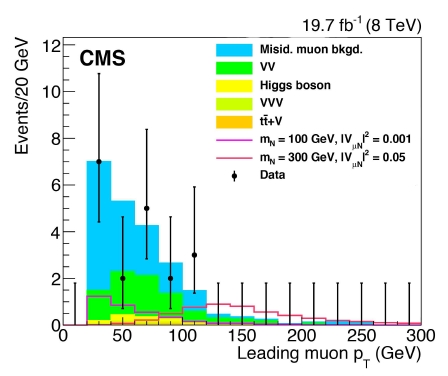
There is another thing I would like to discuss of the graph above. You can see that the error bars are plotted for all bins in the considered histogram, even when there is no data (the points at zero are not explicitly drawn, but that's really a minor detail on which aesthetic opinions differ). Now, there are two schools of thought on whether this is sound or not. Some argue that error bars on bins with zero entries "clutter" the graph and add no information; others argue that they are as important as those on data with more than zero entries per bin.
I belong to the second group. I believe that treating asymmetrically an event count of zero and an event count larger than zero is unmotivated - the two provide equivalent amounts of information. The error bars are a way to guide the eye in a comparison, and leaving aside information in such a comparison is silly.
You should realize that when we draw data in a histogram as points with error bars we are doing two things at once: we are giving information on the amount of observed data (the point), and we are also showing our estimate for the location of the true rate within the bin, by drawing the error bar. The bars you see in the graph above are asymmetric around the point because they are drawn according to the Garwood procedure, which is the most principled way to do it, for Poisson-distributed data. I won't explain what the Garwood procedure is in detail (it amounts to inverting the Neyman construction for the Poisson), but I will indeed mention that it is a central interval, i.e. that the bar extrema span the region of unknown true rate such that equal probability is covered on both sides of the measured rate. The equivalence of "best estimate" for the true rate and observed rate is an implicit datum in the display of point and error bar, by the way.
So, leaving those technical details above on a side: are you in favor of those cluttering error bars or not ? In the example above I agree that they do not provide a lot of information, but there are cases when not plotting them would result in a graph that gives the wrong impression that the data is not in good agreement with the prediction, when the latter is instead the case...


Comments