

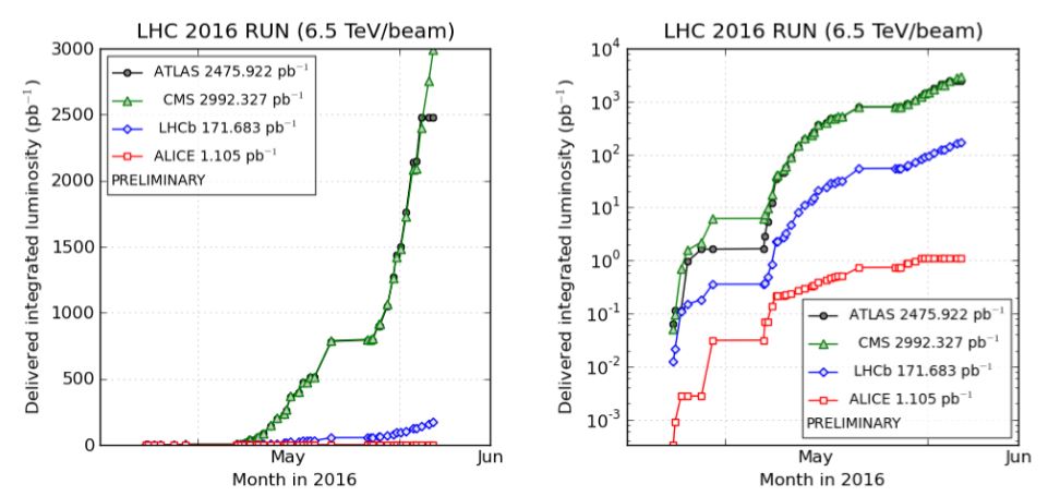
The plot below shows the integrated luminosity that the machine has delivered until the end of may to the four experiments in 2016. As you can see, the rate of collection has increased sharply in mid-May, when the LHC started to get filled with as many as 2000 bunches of protons per beam. This has resulted in the last few days (not shown in the graphs) in the collection of about 350 inverse picobarns (labeled "pb^(-1)" in the graphs on the vertical axes) of data delivered per day to CMS and ATLAS; and much less to the other experiments, LHCb and ALICE, which are however not meant to collect all the collisions that could in principle be produced there.
Okay, you get the gist of it - there's a curve of luminosity versus time, and the slope is growing as time progresses. But what does it really mean, that's another matter. What is a inverse picobarn, anyway ?
I think I have explained the concept in this blog several times in the past already, but I still find it useful to repeat the concept now and then.
So, the inverse picobarn.
The inverse picobarn is a useful measurement unit of integrated luminosity for a modern-day collider; as such it can be used to gauge how many collisions of a certain kind have been produced. I can try to explain this with an example. Imagine a monkey shooting at random with a rifle for a certain amount of time. If you are in the line of fire you might be interested in knowing how many bullets are shot per square meter before the monkey is removed from its post. Call that number L: a number of bullets per square meter L=0.0001 could be an acceptable risk, while a value of L above a few tenths would mean you are in very serious danger of being killed.
We can push this further and be quantitative for once: if you know L and you know the area A of your body, you can easily compute what is the expected number of bullets that should hit you: this is N=L*A. Using relatively simple statistical methods, from N you can then derive the probability of getting hit once, or twice, etcetera. You can even compute the probability of N shots on your right leg, if you really need to - just plug the area of your leg as seen from the muzzle and you are done.
In the above example, the "number of bullets shot per square meter" at your location (i.e., at your distance from the monkey) is really the number you want to know. In particle physics this is the equivalent of an "integrated luminosity", call it L, of some dataset of collisions. The "effective area" of a proton, as seen from another proton, is a number we call "sigma_total" - the total cross section of the proton-proton collision. This is much, much smaller than a square meter: it is in fact about 10^(-31) square meters, if the protons have the LHC energy. A proton's apparent area is, compared to a square meter, about as large as a blood cell on the Sun's surface.
Given that we are working with such a small effective area where collisions may take place - one much, much smaller than that of your right leg- it is not strange that an integrated luminosity of "one hit per square meter" would not suffice to create a proton-proton collision. We need the integrated luminosity to total ten thousand billion billion billion hits per square meter to predict one expected hit!
In order to avoid fiddling with hard-to-spell numbers, it is convenient to quote L in a better measurement unit than hits per square meters. Using "Hits per square nanometer" would be better - we would then win a factor of 10^9 squared, getting rid of two of the "billion billion" in the above sentence. But if we count area in "barns" and luminosity in "inverse barns" - where a barn is an area of 10^(-30) meters - we are even better off: given an effective area of 0.1 barn and a luminosity L equal to one inverse barn (one hit per barn) means you expect N= L*A = 0.1 barn * (one hit) / [1 barn] = 0.1 expected hits!
I hope you noted how to express mathematically "one hit per barn" I had to put the barn at the denominator of the expression: "1/barn" is the mathematical way to express the locution "one per barn", so that when you multiply by a number of barns you get a pure number - the number of hits.
N = L * A... This is not rocket science
Now I think you are closer to appreciate what an integrated luminosity of three inverse femtobarns mean: as the femtobarn is a millionth of a billionth of a barn (the prefix "femto" stands for 10^(-15) in fact), three inverse femtobarns of proton-proton collision equate to N = 10^-1 barns * 3 / [10^(-15) barns] = 3*10^(14) collisions! That's the number of events produced in the core of CMS and ATLAS by the LHC collider this year... Until a couple of weeks ago, that is.
Finally, if you got this down let me also note that the "interesting" physics processes that CMS and ATLAS look into are not ones occurring every time there is a collision between a proton and another proton.
Physicists assign different "cross sections" to different reactions that may or may not take place. These are usually far south of the total cross section: the production of a top quark pair, for instance, has a cross section of 800 picobarns - 8*10^(-10) barns. And the cross section for producing a pair of Higgs bosons (a process I am currently studying) is of 37 femtobarns. How many such events do I expect in the current 2016 CMS dataset ? N = 37 fb * 3 /fb = 111 events! Doh, it's as simple as that... This is not rocket science after all!
What to expect for ICHEP
I believe that if the machine keeps delivering at this pace, by mid-July CMS and ATLAS could have in their hands some 10 inverse femtobarns of 13-TeV collisions. Those data, three to four times larger in size that what was collected in 2015, should spell the final word on the diphoton resonance feeding frenzy that has taken place in the theory community since last December's data Jamboree at CERN. For the probability that a 3-sigma signal is seen in the new data at 750 GeV is... Well, 0.13%, as it has always been. If the 750 GeV thing is real, one should expect to see a much larger signal than in 2015, so we will pretty much be able to draw a conclusion. Or maybe not - statistical fluctuations are always a possibility!


Comments