

But let's go in order. First I owe you a quick-and-dirty explanation of what is the top asymmetry and why you might care about it.
The top pair production asymmetry is a property worth studying in detail at hadron colliders, as it may betray a shortcoming of our theory (the standard model) in understanding and modeling the production, if there is new physics connected with the hard subprocesses giving rise to top pairs. Why do we focus on top pairs and not lighter quarks ? Because top quarks are very easy to identify nowadays, while lighter quarks are much harder to "tag"; but also, crucially, top quarks are the heaviest particles we know. This is taken as an indication that they might have more connection with new physics processes that "turn on" at large energy.
An asymmetry in the production process yielding a pair of top quarks at the LHC can be observed if there is a kinematic difference between final state products of, say, positive electric charge with respect to particles of negative electric charge. Top quarks are charged (they carry minus two-thirds of the electron charge), and their decay "transfers" to their daughters this information, in the sense that the kinematics of the top quark propagates to the kinematics of the decay products. So by counting how many positive and negative charged leptons go toward the direction of one beam or the other, we can construct an asymmetry.
If, as ATLAS does, we rely on the dileptonic decay of top quark pairs (that is, the one where both the top and the anti-top decay to lepton-neutrino-b quark triplets, so that the final state includes two charged leptons, two neutrinos, and two b-jets), an asymmetry in the lepton kinematics can be defined as follows: first define the quantity Delta as
Delta = |eta(+)| - |eta(-)|
where eta is the pseudo-rapidity of the particles, a monotonous function of their angle with respect to the beams direction (beam lines have either -infinite or +infinite rapidity, and particles emitted orthogonally have null pseudorapidity). Then you can form the ratio A_ll:
A_ll = [N(Delta>0) - N(Delta<0)] / [N(Delta>0) + N(Delta<0)].
This quantity tells basically whether the pseudorapidity distribution of positive-charge leptons is broader (A_ll>0) or narrower (A_ll<0) than that of negative-charge leptons. The subscript in A is a double L, indicating we are discussing the asymmetry in the leptons - which is connected to the one of top quarks but is not the same thing. In fact, the latter can be inferred from the former.
At this point you might ask a question: "Why on earth do we expect A_ll to be different from zero, given that we have protons coming in from both positive and negative rapidity directions ?".
This is a good one. Indeed, at leading order in quantum chromodynamics one does not expect any difference. However, we are smashing against each other protons, which are positively-charged bodies. In such collisions the top quark pairs can be produced both by quark-antiquark annihilation (15% of the time at the LHC) and by gluon-gluon fusion processes (85% of the time). The latter process exhibits no asymmetry whatsoever, but the former does, as the positive-charged lepton "remembers" the asymmetry in momentum existing between positive-charge quarks and negative-charge quarks that annihilate. The fact is that the latter carry on average a smaller momentum fraction than the former, due to the way the proton shares its energy among its constituents. That is the source of the small asymmetry measurable at the LHC.
Now, ATLAS extracts an almost-pure sample of dileptonic top-pair decays from events featuring two electrons, or an electron and a muon, or two muons. All of these leptons, if energetic and isolated from other particles, are a nice "tag" of top pair decays - there is little else that can produce them that way.
There are a number of subtleties in determining the A_ll value described above in the analysis, and even more are needed to translate that value into the corresponding "parent" asymmetry between the top and antitop quark. The transition from A_ll to A_tt requires you to reconstruct the top decay kinematics, which is tricky as two neutrinos have escaped the detector without telling us where they are directed toward Vladivostok or Buenos Aires. But it can be done, with some statistical magic connected with weighting events based on the kinematics of the bodies you can actually observe - leptons and jets.
In the end ATLAS produces a measurement of the small asymmetry which is very good - competitive with state-of-the art knowledge - and compatible with the standard model prediction: A_tt is measured as 0.021+- 0.025 (stat) +-0.017 (syst). So what do I have to complain ?
Well, not much, really; rather, I wish to make a small note to my colleagues. The results of ATLAS are obtained separately for the three final states of top quark pair decays - dielectrons, dimuons, and electron-muon samples. Then the three asymmetries are combined using the BLUE procedure (basically a chisquare-based, linear, unbiased estimator). And there's the rub: to run, BLUE requires you to provide an estimate of the correlation between the uncertainties of the input measurements.
Authors write in the paper that they assume all but a few of the considered systematic uncertainties to be 100% correlated. This is not further justified, but looks like a "conservative" assumption - usually by considering uncertainties correlated you keep the final uncertainty in the average larger than if the uncertainties are considered independent on one another. But that is actually not always so!
To understand what might happen let us consider a very simple case. You have two measurements x1 +- σ1 and x2 +- σ2, with, say, σ1<σ2. Let us also say that the two uncertainties have a true correlation level of 50%, due to the fact that they are estimated using similar methods in the two channels. Unfortunately, you do now know precisely that 50%; you know it is sizable but have little means to estimate it correctly.
The two inputs look compatible so you average them, and to be conservative, as you do now know the correlation between the systematic uncertainties, you claim them to be 100% correlated: this must be "conservative", right ? The σ1, σ2 numbers above are assumed to be the combination of statistical and systematic uncertainties; assuming 100% correlation in the systematics brings your estimate of the correlation coefficient in the total error to be larger than what it really is. But as above, you expect this to be conservative.
Upon combining the results -using BLUE, or just writing with pen on paper the covariance matrix, you obtain the following: first you write the covariance matrix V in terms of uncertainties and correlation coefficient; then you invert the matrix and write a chisquared; and finally you minimize the chisquared, obtaining the weighted average x and the (inverse) variance 1/σ^2. The steps are shown below.
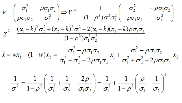
Above, ρ is the assumed correlation coefficient. If the ρ you assumed is larger than the ratio between the total uncertainties σ1 and σ2 (ρ>σ1/σ2) two unsettling things happen. The first is that one of the two input measurements receives a negative weight in the combination: (1-w) is negative. Hence the average ends up outside of the [x1,x2] interval, on the side of x1; x<x1. This is a well-known fact and should raise no eyebrows: when two measurements are very correlated, they tend to "go along" with each other; the true value is most likely outside the [x1,x2] range. I discussed and explained this fact in another post a while ago (very advisable for you to read it, as it is an easy explanation).
The other unsettling thing is more a concern. If you examine the expression for the inverse total variance, you notice that if ρ>σ1/σ2 is increased, the total variance decreases! (It takes a minute to plug in two values and verify this). Let us stop and think at this for a second.
We started by saying that we overestimated the correlation coefficient to be on the conservative side. And we end up with a weighted average which carries a smaller uncertainty than if we had assumed a smaller correlation. What the heck, if this is not trickery then tell me what it is!
The fact is unfortunately true and forces me to say that people that like sausages and people who believe in weighted averages should not ask how they are made. In the case of the top asymmetry the ATLAS folks have been lucky: their result is within the bounds, and all three inputs have positive weight. But as they defined the correlation before they set out to average the inputs, they could well have ended up with one weight being negative; in which case, their "conservative" choice of a 100% correlated systematic uncertainty would have resulted in a underestimated total uncertainty - which is a mortal sin for an experimental physicist.
So, in summary: analyzers, beware. "Conservative" is not always good; actually, it is never good - it is better to estimate things to the best of one's knowledge and understanding, than to "stay on the safe side". Ironically, in weighted average this may put you in the danger zone!


Comments