

Yet the topic is of considerable complexity: it might actually be considered cutting-edge particle physics, in the sense that the techniques used in the analysis are quite advanced. But I love to simplify complex problems to (try and) make them understandable, and it was a quite interesting challenge for me to explain the above calculation to the students today. I think I did it with some success, and I now wish to bring the challenge one step further, and make the solution of the problem understandable for my readers here - that is, for you. And, if you too like a challenge, read on and let me know how far I can take you.
The hardest mathematical concept we are going to use to complete our task is taking the square root of a number. But we do also need to have a grasp of a few basic physical concepts, so I will start with a few important definitions and clarifications which are preliminary to the quite trivial calculation.
Four basic concepts
1) What is a cross section ? A cross section is a number, which has the units of an area, and whose magnitude is proportional to the probability that a particle collision yields a particular outcome. You need not care about the units, but I will still express cross sections in picobarns. You may call them ablakazoons if you prefer; the result will not change.
2) What is "integrated luminosity" ? Integrated luminosity is a measure of how many protons and antiprotons were smashed against one another in the core of the detector. Integrated luminosity, too, has units. It turns out these are inverse picobarns, but you may stick with inverse ablakazoons if you prefer.
3) You may also hear me speak of a "branching fraction", also known as "branching ratio". A branching fraction, or ratio, is just the probability that a particle decays in one particular way; as all well-behaved probabilities, it is a number between zero and one. Nothing hard to figure out, really.
4) Efficiency is another number we need. It is the way physicists call the fraction of successes. For instance, if I say that the electron identification efficiency is 50%, I mean to say that every second electron will fail to be correctly identified by the detector.
The calculation
Ok, that was not too hard, was it ? Let us now try to compute the Higgs boson cross section limits that the CDF experiment should set by looking at WW candidate events in an integrated luminosity of four inverse ablakazoons -more or less what they have in their hands as we speak.
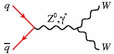 To calculate an expected limit on Higgs production with a decay into W boson pairs, we need to compute the backgrounds we expect to collect in our selection of Higgs candidates. These are for the most part due to the standard model production of W boson pairs (with no Higgs boson involved), through the processes shown in the two graphs on the right above and on the left below.
  So we will neglect other sources of events. Our analysis involves the following steps:
1) select events with two electrons, or two muons, or an electron and a muon; these dilepton events are the result of the decay
2) select events most likely to be due to Higgs decay, with the use of a Neural Network -an algorithm which simulates the workings of neurons in a brain, and can be "trained" to distinguish events of one particular kind. Let us imagine a Neural-Network-based selection which has an efficiency of 80% on signal events, and 10% on backgrounds (that is pretty good, but not too different from reality).
3) count the events we have selected, and compare the result with the number we expect to collect from standard model sources alone.
4) the comparison above, if it is not producing any excess of events, can be used to extract an upper limit on the number of signal events that may be present in the data, given that we have not seen any excess from the expected background rate.
5) From the maximum allowed number of signal events present in the data, we may calculate the maximum Higgs signal cross section which is not incompatible with our counting experimnet.
Now that the path is clearly drawn, let us follow it in good order. We know that the cross section for standard model production of a W boson pair is roughly 10 ablakazoons. Multiply this by the integrated luminosity of 4000 inverse ablakazoons, and you get the number of WW pairs produced in the core of the detector during the data taking we have considered: 40 thousand, give or take a few thousands.
Now let us compute how many of those 40 thousand yield a pair of electrons: we need to multiply by the square of the branching fraction of W decay into electron, which is one ninth. Why the square ? Because we have two W bosons requested to yield electrons, duh! So 40,000 times 1/9 times 1/9 is roughly 500 events. If now the electron efficiency is 50%, we remain with 500*0.5*0.5 = 125 events which we should have collected as "good dielectron candidates". Again, we have taken the square of the electron efficiency, given that we need to pay the price of our imperfect electron detection twice.
A similar calculation could be done for the dimuon final state: nothing changes except the muon efficiency, which we have taken to be 60%: the square of that, divided by the square of 50%, is the increase of dimuon events with respect to electron events. We end up with an estimate of 180 dimuon events.
Finally, for the mixed "electron-muon" case, we have to be careful: there are two ways by which we may get the two W bosons to yield an electron-neutrino and a muon-neutrino decay. The first W may go to an electron-neutrino final state, and the second to muon-neutrino; or the opposite. So we double the electron number, and then multiply by 60% and divide by 50% to account for the larger muon efficiency. If you do 125 * 2 * 0.6 / 0.5 you should get 300 as a result.
Let us take stock: we expect to have collected in our data a total of 125+180+300 = 600 events with the required dilepton topology. Now, the selection with our well-trained Neural Network, which we expect to have a 10% efficiency on the standard model WW background, reduces the sample to 60 events.
We are almost done already! These 60 events we expect to find are due to backgrounds. Now, imagine we do the experiment and we find exactly the number we expected: 60 events observed, with 60 predicted by backgrounds. I admit this is not very likely, but it is more likely than any other number. In fact, considering this case will lead us to a good estimate of the "expected limit" we may set with 4000 ablakazoons of data in the WW search.
60 events found, 60 expected. Mumble, mumble. How many Higgs events can be present amidst those 60, if on average 60 are expected from backgrounds alone ? Well, that is not exactly the right question to ask. What is best to figure out, instead, is what is the largest number of Higgs boson decays which might be present in the data, given that we have not seen a deviation from our expectation.
Here we need maybe the most complex mathematical concept of the whole exercise: the typical random variation of the number of events we saw (60) is the square root of that number, that is roughly 7.5. This is a well-known result of Poisson statistics: on another occasion we could have found 52 events, or 68, or 70, or 48. The probability that we obtained a given number of counts has a Poisson distribution -basically equal to a Gaussian- centered at 60 and with a root-mean-square of 7.5.
The distribution is very informative; actually, too much informative for us: what we need is just a 95% confidence level on the maximum number of Higgs events. This turns out to be about twice the natural width of the distribution, or 15 events. In other words, if I am expecting to see 60 events from background processes, only 5% of the times am I likely to get as few as 45 from the background -which would allow 15 events of Higgs to be present in the data without my noticing. So we may claim that there cannot be more than 15 Higgs events in our data.
What we found above is a limit on the number of events, and we need to convert it into a limit on the Higgs cross section: the inverse exercise to the one we have done above to get the number of expected background candidates.
We know that the efficiency of the Neural Network on Higgs decays should be 80%: then before the NN selection, the maximum number of Higgs decays in the data is 15/0.8, or 18. We also know the effect of the lepton identification efficiency and the branching ratios of W boson decays: it is the same as the one applying to standard model WW pairs, which selected 600 out of 40,000 of them: so the maximum number of Higgs boson decays to WW pairs in the data before the lepton selection must be 18 times 40000 divided by 600, or 1200.
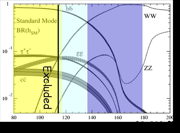 We are almost done: now we just need to account for the fact that the branching ratio of Higgs bosons to W boson pairs is about 90% if the Higgs mass is 160 GeV (a number we obtain by checking the curves shown on the right, which are derived from not too difficult theoretical calculations), and we get the maximum number of Higgs bosons produced in 4000 inverse ablakazooms as 1200/0.9=1333.
 Since the limit of 1333 produced Higgs particles applies to 4000 inverse ablakazoons, we divide by the latter number to get the limit on the cross section as 1333/4000=0.33 ablakazoons: this is according to the master formula which says that the number of events of a specific process is the product of cross section and integrated luminosity.
 And we are done! Our eyeballing estimate of the cross section limit on a 160 GeV Higgs boson that the CDF experiment is expected to set has been found with very simple math, and some approximations. 0.33 picobarns. How far are we from the real cross section expected for the Higgs boson ? That, ultimately, is what determines whether our search is capable of excluding a 160 GeV Higgs or not. Let us check the graph on the right then: for 160 GeV, the standard model predicts (red line, the relevant one for direct Higgs production through gluon fusion) that the Higgs at the Tevatron should have a cross section of 0.3 picobarns -I mean, ablakazoons: whatever is on the vertical axis of the figure. We are very close to the standard model value, but not below it... That means that our search, by itself, is not expected to be able, on average, to exclude a 160 GeV Higgs.
 Conclusions
So, dear reader, as you see there is nothing too mysterious in the results that the Tevatron experiments use to summarize in plots such as the one below, which determines a limit on the Higgs cross section (the full black line) as a function of the Higgs mass, in units of the standard model expectation. Since at 160 GeV the expected cross section is 0.3 pb, and we found a limit at 0.33, that means a limit on R at 1.1 times the standard model: close, but no cigar. By combining our result with similar searches, however, a result such as ours may reach below R=1, such that the Higgs mass may indeed be constrained. That is what happened last spring, when CDF and D0 together announced to have excluded the 160-170 GeV range, by combining their search results.
 In conclusion, I think I have shown that even the apparently most difficult, complicated results of particle physics experiments can be calculated with simple math, if one is willing to sacrifice accuracy for clarity. If you have been able to follow the whole calculation to the end, I would be happy to hear your impressions in the comments column below.


Comments