The inaugural season of intercollegiate football took place in 1869. It consisted of two games: Rutgers played Princeton, and then a week later, they played again. Each team won once, so the “national championship” (awarded retroactively) was split. And despite the schools’ bitter rivalry, the Rutgers newspaper reported an “amicable feed together” after the contests. Since then, the business of selecting a national champion in college football has grown considerably more complex.
Controversy has long come with the territory. In 1932, for example, the national championship was awarded to Michigan via the” Dickinson System” (Frank Dickinson, a professor of economics, devised a ranking system for comparing teams with varying opponent strengths) even though both USC and Colgate went 9-0-0, and not a single point was scored against Colgate all season. To make matters worse, USC defeated 3rd ranked Pitt in the Rose Bowl since Michigan’s conference, the “Big Nine”, didn’t allow postseason games.
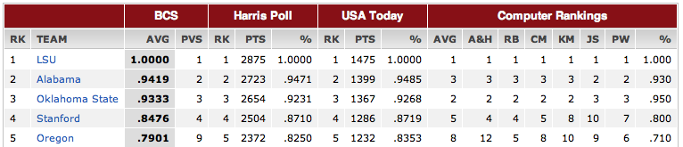
By 1940, Dickinson retired as official ranker of football teams, ceding authority to the Associate Press (AP) poll of sportswriters, which had begun four years earlier. A competing coaches poll started in 1950. Today, a national champion is selected by the somewhat infamous Bowl Championship Series (BCS). The BCS ranks teams by averaging rankings derived from the AP poll (taken over by the Harris Interactive poll), the coaches poll (run by USA Today and ESPN), and 6 algorithmic ranking systems; the top two teams play a single game to determine, once and for all, the national champion.
Still, the BCS remains contentious. Or as Hal Stern, a statistician at UC Irvine says, “from a statistical point of view, the BCS is a bit of a sham.” This year, while LSU is the clear choice for the top ranking, Alabama barely out-polled Oklahoma State for the second spot. But, Alabama already lost (in a close game, 9-6) to LSU earlier in the season, so many fans feel that Oklahoma State deserves a chance.
All this controversy got me curious. What exactly are the ranking algorithms? How well do they work? Maybe I could do better.
If we’re going to talk about assigning values to teams, we need to start by identifying a goal. Ours will be: maximize the prediction accuracy of future games. While this objective may diverge from that of the fans’, as it may in the case of Alabama and Oklahoma State, at least it is easily measurable. The college football season is roughly 15 weeks long (including bowl games); we’ll use the first 7 weeks to predict the results in week 8, then the first 8 weeks to predict week 9, and so on. This sort of rolling prediction, starting midseason, gives the algorithms enough data to make reasonable judgements.
Why can’t we just use the win-loss records? That is, choose the team that has the higher value of wins / (wins + losses) as the predicted winner. We’ll try this as a baseline, and see how much better we can do. But the main problem is that there are 120 division 1-A college football teams in 12 conferences, and each team’s schedule is very different. This is the “strength of schedule” idea. If each team played every other 1-A team, the win-loss record would work just fine; but because they play a particular small subset (typically around 13 games), the win-loss record needs to be adjusted to reflect the quality of the wins and losses.
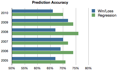
Let’s start with some numbers. This chart shows how predictions made based on win-loss records compare to regression-based predictions (described below). Over 2051 games in six seasons, win-loss predictions average 68.5% accuracy, compared to 72.9% accuracy for regression. The gap is a bit more impressive for out-of-conference games, since the win-loss ratio better reflects a team’s strength in its own conference: 73.7% for win-loss predictions vs. 79.1% for regression (measured across 344 games).
So how can we improve on the win-loss predictions? It appears that most (if not all) of the algorithms developed for the BCS start with the win-loss records and adjust them in various ways, sometimes mathematically justifiable (Sagarin and Colley, for example), and other times not (Billingsley says “I never had calculus. I don’t even remember much about algebra”). But after the PAC-10 complained in 2001 that Oregon was unfairly denied a shot at the national championship, the BCS decided to preclude the use of “margin of victory” in algorithmic ranking. That is, all wins are to be treated equally, whether 8-7 or 50-7. This means that all the BCS algorithms are at a disadvantage.
I can measure the disadvantage by removing the margin from the model. To summarize:
- Win-loss: 68.5%
- Regression model without margin of victory: 70.2%
- Regression model with margin of victory: 72.9%
How does this regression business work? Here’s the idea in its most basic form. Suppose every team has an underlying strength such that the predicted point spread of a game is the difference between the teams’ strengths. Say LSU’s strength is 30 and Alabama’s is 28, so the predicted spread would be 30 - 28 = 2 points.
This description is a model for how games actually play out. Of course in reality, there are players and coaches and strategies and plays and injuries and weather conditions that all effect the outcome of a game. I’m condensing all this into a single made-up thing called “strength”. While this is a pretty drastic simplification, it has the advantage that we can actually do a good job of estimating strength values. This is called “training”: choose the strength values that come closest to reproducing the actual point spreads observed during the season. The beauty of this optimization is that the strength values are derived from a compromise involving all the game outcomes simultaneously.
Here’s a toy example. Suppose there are 3 teams, x, y, and z that play the following schedule:
- week 1: x vs. y result: 21-3
- week 2: y vs. z result: 15-18
- week 3: x vs. z result: 10-42
So we’d like to find strengths Sx, Sy, and Sz such that this quantity is as small as possible:
[(Sx - Sy) - (21 - 3)]^2 + [(Sy - Sz) - (15 - 18)]^2 + [(Sx - Sz) - (10 - 42)]^2
Note that each term in this equation is the squared difference between a prediction and the actual result. The reason we use the squared differences is just because it makes the solution easier to find. This is a standard linear regression, sometimes called “ordinary least squares” because of the squared differences, and it has a straightforward algebraic solution. For the toy example, the solution is x = -4.7, y = -7, and z = 11.7. The version of the equation we need to estimate all the division 1-A team strengths has 120 variables, one for each team, and about 700 terms, one for each game in the season. This is a relatively small learning problem, and my laptop solves it almost instantaneously.
Next, let’s extend the model to include some other factors. We’ll add a variable to represent Home Field Advantage (HFA). We could add an HFA variable for each team, as some teams may benefit more from being at home than others. But this turns out to work no better than the simple version (in terms of predictive accuracy), so I’ll stick to a single HFA variable. Home field advantage, it turns out, is worth something like 3.5 points.
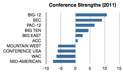
Let’s also add a variable for each conference. This works as a kind of smoothing: there are far fewer conference variables than team variables, so their values should be better estimated. The overall strength is the sum of the conference strength and the leftover team strength. Here are the estimated conference strengths for 2011:
So far, the model assumes that teams either don’t change (improve or get worse over the season) or all change at the same rate. Hal Stern and others have shown that the polls used by the BCS significantly over-value recent results, at least if what they care about is predictive accuracy. But that doesn’t mean it isn’t worthwhile to model change in some way. I found a small benefit from adding a variable for each team that indicates time. Perhaps the simplest way to do this is with a “week” counter. In the first week of the season, the counter is set to 1 for each team, then 2 during the second week, and so on. If a team improves during the season, its time variable will be positive, so that the team’s overall strength increases as the season progresses; team’s that suffer from injuries or get worse for other reasons will get a negative time variable. One small adjustment on this idea is to curve the week counter so that it starts at 0 and approaches 1 towards the end of the season, reflecting the notion that teams change more at the beginning of the season. These features reveal that while all the top 20 teams showed some improvement over the 2011 season, Kansas State and Texas improved very little, while Houston improved the most of any division 1-A team.
There’s one last piece to the prediction story. At the end of November, nobody was quite sure what to make of Houston: they were 12-0, including some impressive blowout wins (56-3 against East Carolina, 73-17 against Tulane), but they’re in the relatively weak Conference USA, and never had to play a very strong opponent. So as far as the regression equation is concerned, Houston’s strength value could well be larger than any other team’s. This defies our intuition: they probably are not really better than once-defeated Alabama or Oklahoma State.
To address this issue we’ll make one small change to the optimization: we’d like to find the set of strength values that reproduce the observed point spreads as closely as possible (as before), but we want those strength values to be as small as possible.
This is called “regularization”. Now, Houston will have the smallest possible strength value that satisfies the regression equation, and in fact, they end up with a reasonable ranking. Here are the top 10, as of December 29th:
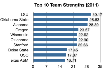
According to our model, then, Oklahoma State may indeed deserve a chance to play LSU for the national championship; LSU remains the favorite by about 1.5 points.
So how do my predictions compare with others? Todd Beck maintains a page that tracks over 50 different ranking/prediction systems, and the system I’ve described here performs close to the top of the list each year. Without doing any more careful analysis, I’d guess it’s at least as good as the best existing systems (note that nothing I’m doing here is novel).
And since it’s bowl season, I’ll conclude with a few predictions:
- The Vegas line favors Oregon over Wisconsin by 6.5 points in the Rose Bowl, but the model predicts Oregon by only half a point: I’d pick Wisconsin to beat the spread.
- Public opinion has soured a bit on Houston since they were upset after going 12-0. The line favors them over Penn State in the Ticketcity Bowl by 5.5, while the model gives Houston a 10.5 point edge: I’d pick Houston to beat the spread.
- As a Cal alum, I’d pick Oklahoma State to beat the 3.5 point spread against Stanford in the Fiesta Bowl since the model favors OK State by 6 points.
References:
- On the first football game: http://scarletknights.com/football/history/first-game.asp
- Dickinson system in 1932: http://mvictors.com/?tag=dickinson-system
- BCS details: http://en.wikipedia.org/wiki/Bowl_Championship_Series
- Current BCS standings: http://espn.go.com/college-football/bcs
- NYT article by authors of “Death to the BCS”: http://www.nytimes.com/2010/10/17/sports/ncaafootball/17score.html
- Hal Stern on college football: http://pubs.amstat.org/doi/abs/10.1198/000313004X2098
- Performance of ranking systems: http://www.thepredictiontracker.com/ncaaresults.php?&orderby=wpct%20desc&year=11