


How do we estimate the confidence range about an estimate? In normal probability theory, we take a distribution and directly measure the dispersion within the data. This dispersion is not influenced by the central location of the distribution, though we see in the previous linked note that the shape and of course scale of the distribution to influence it. Also, we generally think of the typical dispersion sometimes as MAD (mean absolute deviation) and sometimes we think of it as the generally larger σ. Recall that the standard deviation places greater weights on the distribution components, which are furthest from the distribution center.
Now there are some peculiar cases where we can apply the quick statistical √n law, in order to estimate this confidence range. But the way it is liberally discussed across faculties can lead to a false sense that a broader range of physical properties can utilize this √n law. For example, in his book “What is Life?”, the 20th century Austrian molecular biophysicist, Erwin Schrödinger, liberally stated that this can apply “in any physical law” and then also starts with an undocumented presumption that an initial molecular count estimate would follow this √n law. How so? We’ll see in this theoretical note that there are, in fact, serious limits to when we can use the √n law. Let’s start by laying out a few initial, broad examples:
Example A: A total of 480 meteor fragments fall onto Earth, uniformly over a period of several days. As a result of the debris fall, each time zone has an equal chance of being impacted by an equal amount of debris. The average number of fragments per time zone is 20, but is the typical deviation about this average estimate therefore √20, or ~4.5?
Example B: One consumes 2100 calories per day, through 3 fairly-equal meals. The average per-meal caloric intake is therefore 700. Is the typical deviation about this 700 estimate therefore √700, or ~26?
Example C: Each day for a month, a high-end retail store sells one vase. The vase sold could be small and sell for $5, or with equal probability it could be large and sell for $7. Is the typical deviation about the average selling price therefore √6, or ~$2.4?
By the end of this note we’ll be able to articulate which of the above examples, if any, allow for the √n law. We’ll see that the important considerations, one must consider, boil down to these:
• the number of discrete options for the estimate, which we show happens to be connected to dimensions in the physical space and convergence limits towards the √n law, and
• whether the set-up of the physical space is in Bernoulli units or something else, such as nominal, ordinal, or interval numbering conventions.
First let’s show the results from a quick example, in low-dimensional space. Here we only explore the amount of per-meal caloric intake, in just two of the daily meals. We’ll define the dimensions in a short bit. In one case we assume that for each meal there is a 50% chance of consuming 700 calories, a 25% chance of consuming 1400 calories, and a 25% chance of not consuming any calories. In this case, with a binomial, the √n would not work for the per-meal estimate. We’ll describe later how, instead, a √(n/2) law would work.
Now in another case, let’s say that our 700 per-meal caloric intake results from a 1/3 chance of consuming 700 calories, a 1/3 chance of consuming 1400 calories, and a 1/3 chance of not consuming any calories. In this case, the √n would also not work for the per-meal estimate. Though it would work for the total-meals estimate, assuming we do not assume a total estimate and then dependence between meals. In this latter case, the dispersion does not follow the √(n/2) law, but is just of course 0.
So why is there a difference between the two cases above? By spreading the distribution of events among a discrete uniform set of options, instead of a binomial set of options, we in effect work towards the convolution needed to offer the wider dispersion over the options [√n versus √(n/2)].
Here we will work through a specific medium-dimension example to see the convolution properties up close. And then we'll discuss how to expand these results towards a large-dimensional framework. Let's further explore Example B, where a person consumes 2100 calories in 3 daily meals.
Case 1. Binomial, m=2, p=q=1/2
Meal 1: 700 * {0, 1, 1, 2}
Meal 2: 700 * {0, 1, 1, 2}
Meal 3: 700 * {0, 1, 1, 2}
Sum = 700 * 3 * average of {0, 1, 1, 2}
= 2100
Variance = (700)^2 * (3*m)*p*q
= 700^2 * (2*n)/4
Dispersion = 700 * √(n/2)
The 700 are simply a scaling factor and not part of the estimate of n. So this example would not work on a caloric estimate basis, but one could try to continue our analysis could proceed on calories from a total-meals basis. Also while the sum ofn therefore averages to 3, which is 3 times the typical per-meal average, the dispersion is a factor of whatever the scale is. So similar to the 700, we can solve the problem at the total-meals only level, with equal results as the per-meal level. So the √n law is still violated, though we instead see the result follows √(n/2).
Case 2. Convolution
Meal 1: 700 * {0, 1, 2}
Meal 2: 700 * {0, 1, 2}
Meal 3: 700 * {0, 1, 2}
Distribution: 700* 0 → 1 way (0,0,0)
700* 1 → 3 ways (0,0,1 or 0,1,0 or 1,0,0)
700* 2 → 6 ways (0,1,1 or 1,0,1 or 0,1,1 or 0,0,2 or 0,2,0 or 2,0,0)
700* 3 → 7 ways remaining, including (1,1,1)
700* 4 → 6 ways (2,1,1 or 1,2,1 or 2,1,1 or 2,2,0 or 2,0,2 or 0,2,2)
700* 5 → 3 ways (2,2,1 or 2,1,2 or 1,2,2)
700* 6 →1 way (2,2,2)
Sum = 700*3
= 2100
Square Dist.: 700* 0 → 1 way
700* 1 → 3 ways
700* 4 → 6 ways
700* 9 → 7 ways
700* 16 → 6 ways
700* 25 → 3 ways
700* 36 →1 way
Typical sum^2 = 700 (0*1+1*3+4*6+9*7+16*6+25*3+36*1) / (count of all ways)
= 700 * (297) / 27
= 700 * 11
Variance = 700^2 * 11 – 700^2 + 3^2
= 700^2 * (2)
Dispersion = 700 * √2
< 700 * √n
We put aside the 700 for the same scaling rationale as given in Case 1, and thus immediately shift away from this being acaloric-estimate level. At a total-meals level though, we then see the result of √2~1.4, which is under √(n=3)~1.7 versus the less conservative √(n/2=3/2)~1.2. As a result this discrete uniform convolution approach, we show that this case better fits the √n law but still not at the caloric-estimate level.
Before we explore how this approach above works for a broader set of options (or dimensions), estimates, and sampling number conventions, let’s explore why the dispersion is larger for the convolution idea [√n] versus the binomial approach [√(n/2)].
With the convolution approach only we are setting the overall physical space expectation upfront, and more importantly we are evenly distributing the data along the discrete partitions. Therefore not only is there not a larger tendency for each sample to be near the center (e.g., the mound-shaped binomial), but the data presupposes that the sample distribution is not always independent of one another and therefore the variance of the final partition can be large.
Let’s see this for the initial daily caloric sums of 0, 700, and 1400. Under Case 1, the probability associated for each caloric sum is: 6C0/2^6=2%, 6C1/2^6=9%, and 6C2/2^6=23%. And under Case 2, we borrow from the combinations solved above and show it is: 1/27=4%, 3/27=11%, and 6/27=22%. So we see in the chart below that Case 2 has a larger outer probability, while in Case 1 we have a smaller outer probability.
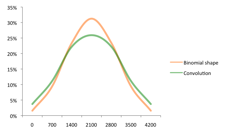
In terms of combinations, there are a greater proportion of ways to get to 1400 or less daily calories in Case 2. And this difference continues with a lager number of options or dimensions as we converge towards the wider √n law. Why is this? It is because it gives equal weight of getting to 1400 calories through eating one meal that day with that meal being 1400 calories, and through eating two meals that day with each being 700 calories. Relative to Case 2, in Case 1 the formula diminishes the weight of the option where one only consumes one meal with that meal being 1400 calories.
One can see these additional three options in blue where only two 700-calorie meals are consumed for the entire day, which add to the three options in red of only one 1400-calorie meal is consumed for the entire day. See chart below for the convolution of 1400 calories consumed in total, from the three meals.
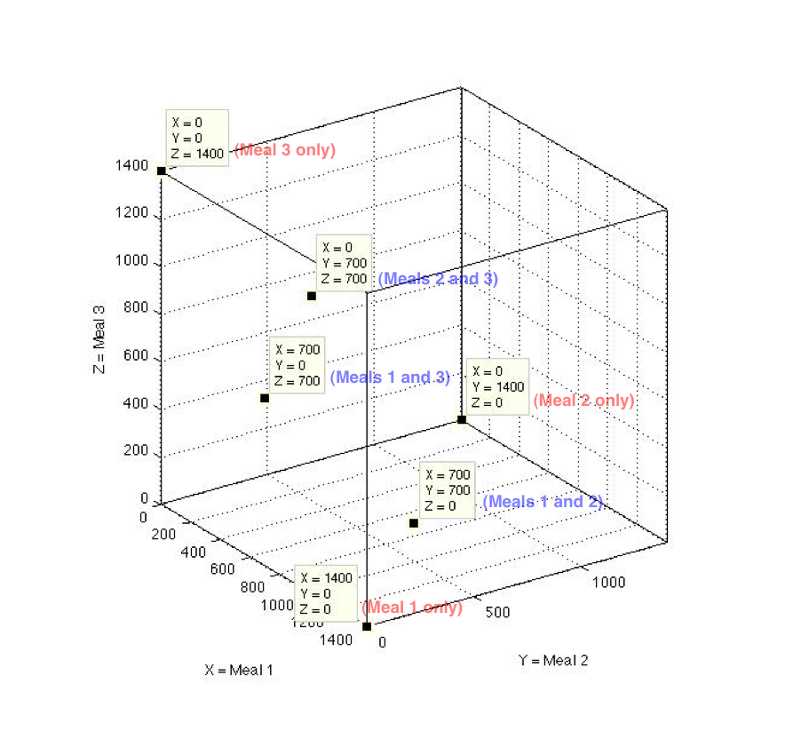
One can see these additional three options in blue where only two 700-calorie meals are consumed for the entire day, which add to the three options in red of only one 1400-calorie meal is consumed for the entire day. See chart below for the convolution of 1400 calories consumed in total, from the three meals.
This form of convolution is important when answering risk questions as well. For example, say that one has a $100 investment at the start of the year. And we know there is a 10% monthly chance that the investment would suffer one loss in that month. And we know that 25% of all losses are at least $10 or more. Does this imply that one would lose at least $10 only 3 times every decade (10 years*12 months*10% chance*25% of losses)? No, because we did not mention what happens in the other 90% of monthly chances, or in the other 75% of the loss levels. Say we suddenly know that there were also a 10% monthly chance that the investment would suffer two losses in a month, and 75% of all losses are at the $5 level. Then we would lose at least $10 in an additional 12 additional months every decade (10 years*12 months*10% chance*100% of losses). So now 15 months every decade would see a loss of $10 or greater.
This is how the convolution probabilities set-up would look like thusfar for the risk example above:
Number of monthly losses = {1 at 10%, 2 at 10%, and unknown at 80%}
Level of losses = {$5 at 75%, and $10 at 25%}
The one loss per month or two losses per month is a risk loss analog to our illustrated Case 2 above. Where then we were considering the number of meals consumed and the per-calorie level of those meals.
Also note that we took the three partitions and showed the resulting distribution in a 3-dimensional chart. This was key since the “physical laws” mentioned by Erwin Schrödinger would generally apply to estimating 3-dimensional molecules in a 3-dimensional space, and thus we must have at least that many discrete partitions or options in our probability distribution. Also nothing would preclude us from thinking about dispersion of estimates across any number of dimensions however, and in fact as we suggested earlier, as this number of options or dimensions increases, the closer to we can potentially approach the √n law.
To wrap up the other considerations, we note that with the risk example and Example B (dealing with meal caloric estimates from convolution), the √n law not work on the actual estimate. But it can work on a number-of-partitions level.
And note that in Example C, the vase retailer could not use the √n law. In this example, the pricing units are $5 and $7, which average to an n of 6. Though that would come with an inherent narrow scaling, which could be modified similar to Example B where we simply relocate the distribution options’ lower bound from $5, to $0.
So Example A is the only one of the three that can simply use the √n law. A lesson learned that while it is easy for scientists and risk managers to take a probability short-cut, rename it a broad physical law and thereby use it liberally, this is a case where the fundamentals probability theory require the user to take better care in thinking through their estimate’s confidence.


Comments