Here is the concluding part (for the first part see here) of a discussion of a few subtleties involved in the extraction of small new particle signals hiding within large backgrounds. This is a quite common problem arising in data analysis at particle physics experiments, but it is not restricted to that field. Quite on the contrary: narrow Gaussian signals are commonplace in many experimental sciences, and their identification and measurement is thus an issue of common interest.

I have to warn you, dear readers: many of you will find the discussion below quite boring. If you have no interest in basic statistics or in the issues connected with data analysis, parameter estimation, or signal searches, you are certainly advised to pick another of the dozens of interesting articles this site contains. In all other cases, please stay with me, since this post will teach you something you might not find elsewhere.

Introduction

Despite the generality of the problem, here I will stick to thinking in terms of the particle physics problem, i.e. the extraction of a resonance. However, you will find out that my conclusions are independent of the specific nature of the signal. In fact, it applies even to non-Gaussian signals!  
 
I also wish to repeat straight away what I mentioned at the end of the former installment of this piece. The results I am about to discuss are unpublished, since they have only appeared in a internal document of the CDF collaboration, ten years ago. They are thus unknown outside of CDF, and they constitute "original research" -although quotes are necessary, given its rather scarce value; in any case, they are my very own cooking, and I stand by them as I do with any other result of my research.

Actually, the secrecy of the results is so well kept that, regardless of the internal document I wrote on the topic ten years ago, even my CDF colleagues seem to have forgotten it, or most likely never heard about it. Of course: CDF has an archive of about 10,000 internal documents that date as far back as 1985 or so, and it is perfectly impossible to know all of them.

I had a direct proof of the oblivion in which my study had fallen a few days ago when, in the process of reviewing a CDF draft paper (reporting on a quite striking and beautiful new result, one which I hope I will be able to discuss here in a few weeks), I found out that they had neglected to properly account for the effect. Of course, I urged them to read my old document: this tickled my ego -a small benefit of being the chair of the review committee.

A bit of particle physics

When an experimenter sets out to search for a bump in a smooth mass distribution, the business he or she faces is always the same -it has not really changed significantly since the birth of subatomic physics. One constructs a suitable model for the shape of background events -possibly using independent sets of data where a signal is not expected- and then attempts to fit the observed distribution as the sum of background and a narrow Gaussian bump, the latter representing a possible new particle signal.

Incidentally, besides trusting one's background model, one must of course make a hypothesis for the mass shape that a unknown signal might display in the data. Here two things come into play: the physics of the interaction causing the disintegration of the particle, and the physics of the detector measuring the decay products.

If the particle has a decay mediated by strong interactions, which are strong and thus act fast, the resonance shape may be wide, because the shorter a particle lives, the least well-determined is its mass. Ever wondered why when a bass tone is played for a short time on a piano you are unsure on its exact pitch ? That is because you have not heard a sufficient number of repetitions of its vibrations: low notes have smaller frequency, and a short note may fail to yield a sufficient number of vibrations. Similarly, the mass of a quickly-decaying resonance is not quite well determined, so when you add together many decays, you get a wide distribution, centered on the mass of the particle. Its shape is not perfectly Gaussian (if you really need to know, it is a Breit-Wigner function convoluted with a Gaussian, save for subtle deformations whose discussion belongs elsewhere), and the width of the distribution may then provide a measure of the lifetime.

As opposed to a strongly-decaying resonance, a particle undergoing a decay mediated by weak interactions (that is, due to the emission of a virtual W boson) has a very well-constrained mass: it lives orders of magnitude longer, and its mass is thus forced to match exactly the nominal value. What one observes in that case on top of the background is a narrow Gaussian shape, whose non-zero width is only due to the finite resolution with which the momenta of the decay products are measured by the detecting apparatus.

Statement of the problem

Let us now forget about particle physics and take in consideration a "standardized" search for a strictly Gaussian signal in a mass distribution, and let us take the background to be flat for simplicity; the results we will find are qualitatively insensitive to these simplifying assumptions. On top of that flat background we search for a Gaussian signal of fixed width: we assume, that is, that the particle decays weakly, so that the width of the signal is fixed to the well-known resolution of our apparatus.

What we are looking at is a situation like the one described by the graph on the right, where is shown the example of a 100-event Gaussian signal of unit width (in our favourite units of measurements, the gudungoons), sitting on top of a background flatly distributed between -5 and +5 gudungoons, and amounting to 1000 events. These are the two shapes that our fit program knows -their sum is what what it tries to interpolate the data points with.

Now imagine you generate a histogram with 1000 entries picked at random between -5 and +5 gudungoons: these will make a flat distribution, if you random number generator is not playing tricks. You take the resulting distribution and attempt to fit it with a minimization routine of your choice (I used stand-alone MINUIT in my studies 10 years ago, but using it within ROOT does not change matters). In the situation we have put together, the fit will only have three free parameters to adjust in order to find the best interpretation of the data: the size of the flat background (say its integral in the fitted region), the size of a hypothetical Gaussian signal sitting on top of it (again we can take its integral for simplicity), and the mean of that Gaussian. What is going to happen ?

It is easy to answer the question without doing any math. On average, the fit must return a value of zero signal, because we did not put any of it in the distribution. So the average value of the total background returned by the fit will be 1000 entries, and the signal will on average amount to zero entries. But is this the most likely outcome ? The answer is NO. The fitter will try to use the degrees of freedom of the Gaussian shape -which it is allowed to move around at values different from zero gudungoons- to explain away a fluctuation of background counts happening here or there on the background spectrum we have generated. We have explicitly asked the fitter, in fact, to use those degrees of freedom to minimize the difference between function (sum of background and signal) and data!

The basic test

If we do a few thousand times -say 10,000- the random generation of a flat 1000-entries histogram, followed each time by a fit of the histogram as the sum of Gaussian signal plus flat background, and we store the results, at the end the result of the fits can be displayed on a histogram showing the returned size of signal which the minimization procedure has found. This is shown on the left: as you can see, the average number of fitted signal entries is zero (within uncertainties), as we correctly guessed; but zero signal entries actually is a very unlikely outcome: the histogram in fact shows that a much more probable situation occurs when the fit returns about 30 entries, either positive or negative. 30 events is about the square root of 1000, and it thus is of the same order of magnitude of the typical Poisson fluctuation of the background.

(What the above means is that when you generate at random a distribution containing 1000 entries, distributed evenly in a given interval, you will get something which is flat only within the typical statistical fluctuations: these flukes have a size equal to the square root of the entries in each bin; however, the global result does not depend on the binning of the histogram, since the fit is to first order insensitive on it: more bins with smaller number of entries collectively act as fewer bins with more entries.)

More interesting is to examine a two-dimensional distribution we can extract from those same 10,000 pseudoexperiments: one showing on the vertical axis the number of fitted entries attributed to the Gaussian signal, and on the horizontal axis the mean of the fitted signal. Each dot in the graph represents a fit to a different generated histogram.

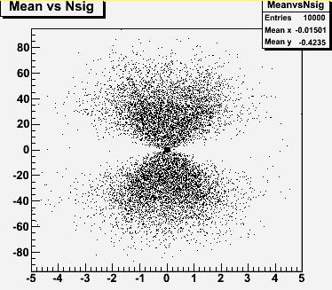Every time a histogram is fit, the program performing the minimization starts its search for a signal with a mean equal to zero, and zero integral, but as the search for a best fit progresses, the Gaussian is moved around, and its integral is made positive or negative, until a stable result is found. What the graph on the right shows is that in order to find larger signals (both positive or negative), the fitter has to move the Gaussian shape significantly away from the starting value.

To prove that it is this "sniffing out" of a fluctuation what drives the fit to extract sizable signals -30 events or even more- from distributions which do not contain any, let us do another experiment. Imagine you now take the same 10,000 distributions generated from background alone, and you fit each of them as the sum of signal and background as before, but this time you fix the signal mean to zero. What do you think will happen this time ?

The fit is now prevented from moving around the Gaussian bump on the spectrum, in order to accommodate a positive or negative fluctuation of the generated background shape happening a few gudungoons away from zero: all it can do is to accommodate a fluctuation exactly sitting at zero gudungoons, nothing more. But such a fluctuation is on average null! If you remember what we discussed in the former part of this post, you will agree that the "look elsewhere effect" grants that a fluctuation is guaranteed to happen somewhere, with a multiplying effect on the probability that a signal is found on the spectrum. By fixing the average of the signal shape, you force the fit to forget about those fluctuations. The result is shown on the left: The average number of entries for the fitted signal is still zero, but zero is also the most probable value for it now!

Add signal, sit back and enjoy

Now that we have understood the mechanics of how a fake signal can be found by our fit routine in a background spectrum, and sized up the possible effect of allowing the mean of the Gaussian to roam around, let us take the case of a 100-entries signal, of standard shape (1-gudungoons width, 0-gudungoons mean), sitting on top of 1000 background entries. This time, that is, we ask the fit to find a real signal. Of course, the result we expect is that on average the fit will indeed return a 100-entries signal. Poisson fluctuations can still happen, but they are typically smaller than 100 events, so we expect the real signal we are generating to drive the fitter in the right spot of the spectrum.

A sample distribution with a fit overlaid is shown on the right (top frame): the histogram has 100 bins, so the 1000-entries of background distribute with an average of 10 entries per bin; a small bump is visible by eye at the center, and indeed the fit has no hesitation to pick it up. If we repeat this experiment a thousand times, we obtain the distribution of fitted signal entries shown on the bottom frame. This teaches us that the fit finds on average 103.7 entries: things work out nicely, it seems.

But wait a minute: 103.7 is reasonably close to 100 when one performs one single fit, but what we are talking about here is the average of 1000 trials: the error associated on the mean of that roughly bell-shaped curve is given by the RMS divided by the square root of 1000-1=999. From the graph we read off a RMS of 23.6 entries, so the error on the mean is 23.6/sqrt(999)=0.75. 103.6 is actually four standard deviations off the average!

A four-sigma effect. Hummmm. An experimental particle physicist usually jumps on the chair upon seeing a 4-sigma fluctuation. Is there something going on here ?

To find out, let us repeat the same test above, but this time let us do 10,000 trials. The mean number of entries attributed to the signal distribution by the fit is now 103.1, and the RMS is 25.2: these results are consistent with those of the former test. But now we have to divide the RMS by sqrt(9999) to get the error on the mean: so it is actually 103.1+-0.25, which is twelve standard deviations away from 100.0!

What we have shown conclusively is that the fit is biased. There is a 3.1+-0.3% bias on the integral of the signal distribution that the fit on average extracts.

The bias is due to the "greed" of the signal degrees of freedom of the function we use to fit the histograms: the Gaussian shape moves around from zero, even in the presence of a steady 100-event bump, to pick up the most advantageous fluctuation happening left or right of the 100 signal entries. Both moving away from a negative fluctuation, and toward a positive one, are ways by which the Gaussian allows for a better fit. And both increase, on average, the number of fitted signal entries returned by the fit. The real reason why the fit behaves this way, however, is hidden behind the details of the minimization function, but a discussion of these details goes beyond the scope of this post.

Studies of the Greedy Bump Bias

Once we have established the presence of a bias, we may as well decide to size it up once and for all: so let us try to establish whether the bias depends on the amount of background sitting underneath a 100-entries Gaussian bump, by varying the background size and performing 1000 fits each time. The results are shown in the figure below.

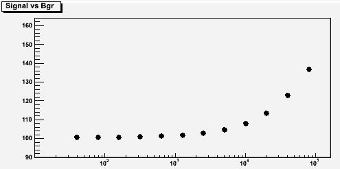On the vertical axis of the graph you can read off the average number of fitted signal entries, and on the horizontal axis is the number of background events that have been generated. You can see that, when the background is not large, the fit behaves well: the resulting signal found is then always compatible with exactly 100 entries. However, if the background becomes large, its fluctuations become important, and the effect -the greedy bump bias- gradually becomes important.

What I have shown above is the case of 100 signal entries, for a varying background. A reasonable question one might then ask is whether the bias scales with the amount of signal in the histograms. Let us then try a case with 200 signal entries. The results are shown below, this time in red. The meaning of the axes is the same as those of the former graph.


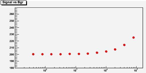
Again, we are finding a positive bias on the returned signal, when backgrounds are very large. The shape of the bias dependence on the number of background entries is the same -a monotonous growing function-, but numbers do not match: while, in fact, with 100 signal entries we were finding a 7-8% bias if the background amounted to 10,000 entries, now the bias is much smaller. However, we should have expected this: a 200-event bump is stronger than a 100-event one, and thus harder to bias with a background fluctuation. What matters, in fact, is a figure of merit we might call "signal significance", and amounting to the ratio Q between the size of the signal and the square root of the size of the background sitting underneath it: Q=S/sqrt(B). The case 100/sqrt(10,000) has a figure of merit Q equal to 1.0, and so we should compare it with the case of 200 signal entries and 40,000 background entries. Indeed, if we do that, we see that the bias is equal in those two cases.

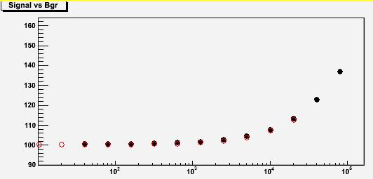
We can thus overlay the two bias versus background curves found above, provided that we scale the signal by two (to match 100 and 200 entries) and the background by four. The result is shown below, and it demonstrates that the bias is universally a function of Q! The red points are barely visible under the black ones... The two sets describe the same function!



There would be many subtleties that I could discuss to add dimensionality to this entertaining problem. However, I feel this post has reached a forbidding length already. If you are interested, we can discuss in the thread below details such as:

• dependence on the input values to the fit function;

• dependence of the bias on the fit range;

• dependence of the bias on whether the user discards negative-signal results;

etcetera... The matter, in other words, is complicated, and it is hardly possible to derive a universal correction factor to apply to any practical case.

What one should do, when fitting a small signal over a large background, is to create pseudo-experiments like I did above, and study how well he can fit a signal under his own special conditions. In all cases, the bias I have demonstrated above is only sizable in extreme cases, when one would not probably venture into trying to fit a signal: it appears only when the background is so large that the significance is negligible in comparison.

To conclude this long and technical post, I would like to add that nowadays, most particle physics searches for small signals do rely on the technique I have used to generate the graphs above: the one of pseudo-experiments. If you know the functional form along which your data distributes, you can generate gazillions of pseudo-distributions, and their study provides a wonderful tool to understand the tiniest subtleties of your methods to extract the signal. For instance, it is with pseudo-experiments that we usually demonstrate the significance of a new signal. I will discuss one such case very soon.

UPDATE: a dummy's guide to study the greedy bump bias by yourself, complete with source code, is here.