

Imagine, for instance, that you collect events with four high-transverse-momentum leptons (electrons or muons) with the ATLAS or CMS detector, and you wish to sort out which of these fit better to the hypothesis of being originated by Higgs boson decay into two Z bosons (with each Z boson in turn producing a lepton pair) rather than to the alternative hypothesis of being due to the incoherent production of a pair of Z bosons -a process that has nothing to do with Higgs bosons. This means you need to classify the data events using their observed features.
In principle, the problem is trivial: if one knows exactly the multi-dimensional probability density function of the signal and background in the space spun by the variables that describe the observed features of the events, then one can classify the data using the likelihood ratio of the two hypotheses, L(x|H1)/L(x|H0), as discriminant. Here L is the likelihood function, x is a vector describing the data to be classified, and H0, H1 are the two hypotheses corresponding to the two classification choices (in our example above, H1 would be "this event comes from a Higgs decay", and H0 "this event is due to Standard Model ZZ production background".
In other words, if you know the probability that x is observed given H1 and the probability that it is observed given H0, the ratio of the two is the highest for the events that fit the H1 hypothesis best. One can therefore use the ratio as a classification tool - for instance, one can order some data according to their ratio, and then take the first ones as those most likely to be Higgs decays.
In practice, unfortunately, one never knows perfectly well the multi-dimensional probability density function of the two hypotheses: there is no parametric form describing it, and all one has is a sample set of events belonging to each of the two classes.
Such samples can be constructed, e.g., by a Monte Carlo simulation which generates collisions according to the known physical processes, passes all produced particles through a detector simulation, and reconstructs the resulting data as is done for real events. But all these operations take a finite amount of CPU, so one is usually very, very far from knowing the density function of the two hypotheses with arbitrary precision.
Typically one works with Monte Carlo samples with one million events, or less. If one then wants to use ten variables to describe the "feature space" that characterize the events -these could be, in our case, the transverse momentum and rapidity of each of the four leptons, plus a couple of azimuthal angles between two pairs- then one will only have a very, very rough description of the density in this 10-dimensional space: for instance, making three bins in each of the 10 variables ("high value", "medium value", and "low value"), the average population of each of these 3^10 = 531,441 bins will be of less than two events !
Working with a "density" described by the presence, in any one of those very coarse bins, of two rather than zero or five events is tantamount to admitting general failure. Say that your Monte Carlo for the background populates a certain bin with 1 event, and the Monte Carlo for the signal populates the same bin with 3 events, can you conclude that data events falling in that bin will have a three-to-one probability of being signal ones ? Of course you can, but how reliable would your conclusion be ?
Very unreliable, in fact. Observing three signal and one background events in that bin means little on the real probability ratio. The odds that the background is actually higher than the signal in that bin, having seen 3 signal events and one background event (out of same, say 1-million, sized starting MC sets for signal and background), is as large as 3/16 ! So one cannot conclude anything significant based on similarly small numbers.
[For a proof: we calculate the probability that s > b (where s and b are the true means of the signal and background in the bin) given that we observe 3 signal and 1 background events, by solving a double integral as detailed below. Note that we have a two-dimensional distribution describing the combined probability of observing three signal events and one background event: this is the product of two independent Poisson distributions. We integrate the two-dim density from zero to infinity in s, and from zero to s in b, so that we only consider the half-plane where s>b.]
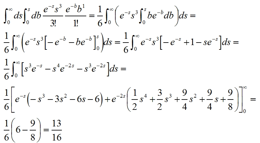
[If you have trouble understanding how the integrals are computed, remember the rule of integration by parts, with which one always solves quickly all integrals of forms like
x^N * e^-(αx) and similar ones.]
Okay, so you realize that it is quite hard to populate meaningfully the space spanned by many variables. And above we have only discussed the case of 10 variables: imagine what happens when you want to estimate a density in a 20-, or 30-dimensional space! This is called in jargon "the dimensionality curse". How to compute our likelihood ratio discriminant then ?
That is precisely the task that the various multivariate algorithms try to address. Of all the choices on the market I like one which a long time ago, an inexperienced young researcher, I "invented" myself (only to discover years afterwards that it was all very well known, including my most witty tricks). This is the so-called "nearest-neighbor" technique (which I dubbed "hyperball algorithm" time ago).
The nearest neighbor algorithm basically estimates the density of a distribution from a finite reference set of discrete events taken from it. It does so by considering the distance, in the multidimensional space, between the point of space where the density is to be estimated and all the events of the reference set. If one has, say, a million events in the reference set, one has a million distances for any point of the space. One can either decide to base the estimate of the density on the number of events within a fixed distance, or weigh the full set with some pre-defined function of the distance. I use a Gaussian "kernel" function for this purpose, but other choices can be made.
Today I was discussing with colleagues in my research group in Padova the need to produce some discriminant for our analysis of CMS data, and the issue of what method to use arose. I was quick to point out that the relative likelihood method, being based on single-dimensional distributions which know nothing of the inner correlations among the feature space variables, is often a poor performer when compared to others, and I offered the nearest-neighbor as a valid, and quick, alternative.
[The relative likelihood has nothing to do with the likelihood ratio! In fact it is a poor alternative: one only looks at the single-dimensional distribution of each of the feature space variables, and computes an estimate of the multi-dimensional density by taking the product of all the single-dimensional densities. In practice one works with histograms: the product of the "heights" of the bins corresponding to the tested point, for all the histograms describing the variables of the feature space, is what one uses as an estimate of the density. It is a poor man's approach, but in some specific cases when correlations are irrelevant it may be a good choice.]
To objections that insisted on the higher simplicity and relatively good performance of the relative likelihood approach, I could only explain that computing a nearest-neighbor discriminant can take as little as twelve lines of code. But then I needed to follow words with facts, and as our meeting ended I set out to demonstrate what I meant.
So I wrote a small piece of code that generates mock data in a multi-dimensional space: according to a uniform distribution for background events, and according to some combination of uniform and Gaussian distributions, partly correlated, for signal events. The program then generates "real data" as a mixture of the two processes, using the same density functions in proportion.
What to do with that data ? Well, one can then compute three different discriminants: one based on the likelihood ratio, one based on the relative likelihood, and one based on the nearest neighbor concept. Note that we have the luxury here of being able to compute the likelihood ratio - the best possible performer - since we know the multi-dimensional pdf of signal and background perfectly, having generated data with it.
The program is available to anybody willing to try it (but you will need to first download the root program from http://root.cern.ch if you do not have it yet, or to convert to a generic C++ program by adding appropriate libraries otherwise) at this link. Below I show some sample results from a run with 50,000 background and 50,000 signal training events, and 5000 events to classify; these contain 80% background and 20% signal.
It is customary to plot the discriminating power of a multi-dimensional discriminant on a double-logarithmic graph where on the x axis is the signal efficiency, and on the y axis is the background efficiency. One has curves in this space which correspond to different values of a discrimination cut on the discriminant. Below, in red is the likelihood ratio, in black the relative likelihood, and in blue the nearest neighbor.
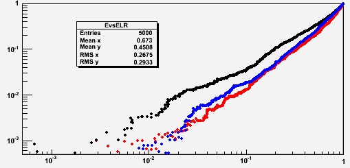
In this particular example (six variables, where background is uniform in the space while signal has four variables correlated in pairs, and two uncorrelated; the marginal distributions are sums of Uniforms and Gaussians) we see that the nearest neighbor manages to classify events much better than the relative likelihood, approaching the performance of the "perfect" likelihood ratio.
In fact, the blue curve is always on the right of the black one: this means that for any value of the background efficiency (the rate at which one incorrectly picks a background event in a selected sample) the signal efficiency of the nearest-neighbor discriminant is higher.
So the message of this longish article is the following: do not neglect correlations - their presence may make a big difference !


Comments