

While providing the results for experts and beginners alike, I will try to make this discussion as simple as possible (but not simpler), something that lately I tend to forget. I do not like my blog posts to be too technical, but maybe I am getting old and my popularization powers are weakening. Let's see.
What it is about
The b quark is one of the six elementary matter particles that respond to the strong force, and bind together in hadrons. You know hadrons well: protons and neutrons are the prime examples, and they make over 99.9% of your own body mass by forming nuclei of hydrogen, oxygen, carbon, and the other stuff that your are build out of. But there are many, many hadrons that can be created out of quark-antiquark pairs or quark triplets. The former are called "mesons", the latter are called "baryons". But I won't be using this terminology any further, so I was just trying to annoy you with some useless information here.
So what is special about the b quark ? Well, it is the second heaviest one. It weighs like five whole protons all together. Physicists believe that there is a mystery to unveil here: the widely different masses of quarks is a puzzle and an exciting research topic. In truth, however, b quarks are interesting because by studying how they are created in energetic collisions we learn a lot about the force that binds quarks into hadrons. b quarks are special for other reasons, too; but I will not discuss these reasons here. Suffices to say that there are multi-billion-dollar projects designed with the sole aim of producing large numbers of b-quark hadrons: BaBar and Belle are past examples, but now there is also SuperB, a new facility that will one day see the light in the suburbs of Rome, Italy.
So let us stick to b production, and specifically, to how frequently and with what characteristics it occurs in the proton-proton collisions produced by the Large Hadron Collider, the powerful new CERN particle accelerator. While physicists could well guess the characteristics of b-quark production in the 7 TeV collisions that have taken place in the core of the CMS and ATLAS detectors from March to November last year, some details were not easy to predict.
Producing b quarks
The proton normally does not contain b quarks. That is, it does, but only for extremely short periods of time: if you take a snapshot, only very rarely will you see a b-quark inside the proton. So it is hard to shake one out of a proton by smashing against it another proton. Much easier is to use the energy of a powerful head-on collision between a quark in one proton and an antiquark in the other: the energy converts into mass, so if there is at least 10 GeV of it -ten proton masses- the chance arises that a b-quark pair pops out.
The fact that 10 GeV is a very small fraction of the possible available energy from a LHC collision -it amounts to little over one per mille of the total collision energy- makes the theoretical calculation of b-production rates complicated, and thus a comparison of predictions with experimental results more interesting. The prediction is complicated for two reasons. Firsth, that in order to compute a predicted rate of production we need to know the probability to find a quark or a gluon inside the proton which carries a very small fraction of the total proton energy; and this is not well known. Second, the calculation at these small energy fractions involves the sum of large factors, which we do not know how to perform precisely.
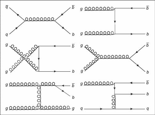
The figure below shows a few "Feynman diagrams" that result in the production of b-quarks in proton-proton collisions. These diagrams describe how the initial-state quarks or gluons (straight or curly lines coming in from the left) collide, and how the energy materializes into the massive b-quarks. There are three different kinds of processes, at "leading order" (that is, in the most simple configurations capable of producing the reaction): direct production (the four top diagrams), flavour excitation (bottom right), and gluon splitting (bottom left). But I won't bore you with this detail here.
A reason to be happy for experimenters is that, despite the smallish amount of data produced by the LHC in 2010 (forty times more data is expected this year!), that is quite enough for some critical comparisons of experimental b-production rates with the predicted ones. This is because these rates are comparatively high! In 7 TeV collisions a b-quark is produced once in a few hundred cases, so in the two trillion collisions produced in the core of the detectors in 2010, one expects tens of billion b-quarks. The analysis reported below just used two thousandths of that data for a meaningful, precise result.
A CMS result: Open B Production Cross Section
One search for such processes was performed by identifying a muon. Muons -heavier copies of electrons- are rare in proton-proton collisions, but they are seen with extreme purity and efficiency by the CMS detector (guess what the M in CMS stands for). Muons are most of the times the result of the decay of a b-quark. By selecting events with muons, one automatically enriches the sample of b-quark decays. Then, by studying the relative momentum of the muon with respect to other particles traveling nearby (so-called jets of particles, produced in the materialization of stable bodies by the fragmentation of the original quarks or gluons created in a energetic collision) it is possible to understand how many of those muons really do come from b decay. This is shown in the graph on the right.
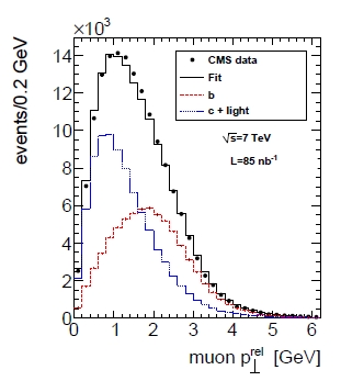 The variable called "Pt rel" is this relative momentum of the muon with respect to the jet. It is larger for b-produced muons (in red), because the b-quark is heavy, and in its decay it gives a larger kick to the muon than other processes do (in blue). A fit to the data distribution (black points) determiines the fraction of b-produced muons in the sample, and from that researchers are capable of calculating the total number of produced b-quarks. Then, this number is studied for different values of the kinematic characteristics of the muons -their transverse momentum (this time transverse refers to the proton-proton beam line, and not to the direction of the jet!), and their angle with respect to the beam. Actually, being such complex bastards, experimental physicists do not use the angle from the beam, which would be too simple to understand. They rather use the "muon pseudorapidity", which is the logarithm of the tangent of half the angle that the muon makes with the beam. Ah, change sign to that once you've computed it. There you go.
But worry not. Pseudorapidity may sound difficult, but it is just a number. The more the muon travels in the beam direction, the larger the number. So let us look at the rate of b-quark decays to muons as a function of muon transverse momentum and as a function of muon pseudorapidity, and check how it compares with theoretical predictions.
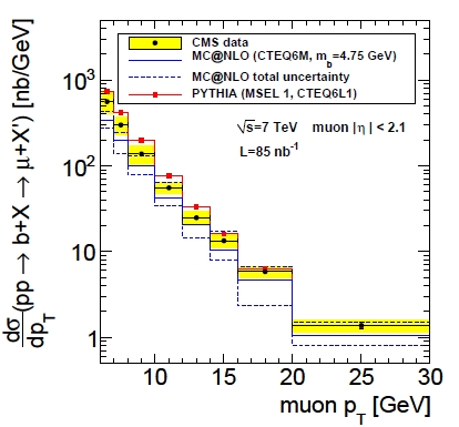 In the graph on the left you can see the CMS data points, with yellow shading highlighting the total uncertainty, compared with two different calculations. The data are presented as a function of muon transverse momentum here: this is a "differential cross section measurement", meaning that it shows the production rate for narrow intervals of the muon transverse momentum. As you can see, the data lies halfway between the MC&NLO predictions (a calculation performed by summing the contribution of many, many possible production mechanisms) and the Pythia predictions (a calculation produced by a computer program that simulates the various phases of the collision and b production processes).
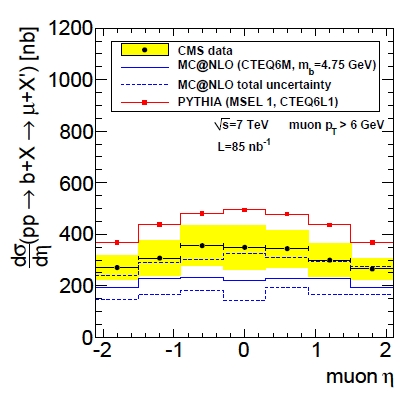
In the other plot, shown below, you see the differential cross section as a function of muon rapidity. Here, again, you see the data halfway between the two predictions. Notably, though, the shape of the differential distribution agrees with the calculations.
What do we learn from these measurements ? Well, from the comparisons we learn that there are important contributions that are not contained in the NLO calculation. The inclusion of "next-to-next-to-leading-order" diagrams (NNLO) in the calculation might, or might not fix the discrepancy. The fact that the disagreement is not only at low pT is an important input, too. But we also learn that the CMS experiment is up and running in important, detailed tests of quantum chromodynamics!
In the next post, if I find the time, I will describe another measurement of b production in CMS, one performed with a different technique - a full reconstruction of B+ mesons from their decay into J/psi K final states. Stay tuned if you are interested in this topic!


Comments