

Your response to my small riddle was quite good, forcing me to provide a timely and exhaustive explanation of what is in the plot I posted a few days ago.
So, the plot (shown again on the right below, but with axis labels this time) shows a rather funny functional form. There are no unit labels on the x and y axes - I removed them because they would have given away the answer immediately. The function is funny because it is made up of vertical and horizontal segments, plus curved links. What on earth does it describe, if not the silhouette of a train (as a reader wittily remarked) ?
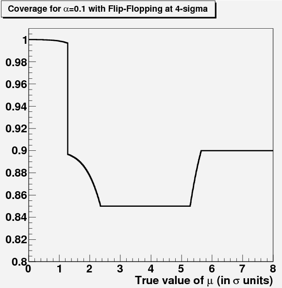 In short and technical lingo, the function describes the exact coverage implied by the setting of a confidence belt on a positive or null parameter measured with unit Gaussian resolution, in case the experimenter avoids null intervals by a lower constraint on the upper limit, and switches to quoting a two-sided interval if the observed measurement is more than four standard deviations away from zero. A reader in the thread (unfortunately an anonymous one) guessed the meaning of the plot quite early on, but later on another (or the same, and unfortunately again anonymous) wrote it most precisely:
"It is the coverage of the confidence intervals obtained for the mean value of a standard gaussian (sigma=1) by the flip-flopping physicist described by Feldman and Cousins . The plot and the quoted numerical inputs imply that such a physicist quotes an upper limit for a less than 4 sigma result of the measurement and a central confidence interval for a result above 4 sigma. The experimenter aims to obtain intervals with coverage always equal or greater 0.9, but actually the flip-flopping policy causes undercoverage below 0.9 for a significant range of values of the true mean value."Ok, ok. I know what you're thinking. Something like "what the hell does this mean???". First of all, what is coverage ? Second, what is a confidence interval ? And third, what is a flip-flopping physicist ?
Let me explain in good order. First very quick definitions to avoid keeping you in the dark, and then I'll develop a bit the concept. Note that this post is not very simple to follow: most of you will not want to know all the details I discuss. Still I thnk it may be worth reading for graduate students doing new physics or astrophysics searches. Ah, and another warning: I am not being rigorous in my definitions, and I might actually err here and there, since I am writing this without checking the books. Corrections welcome.
So let us start with Coverage. Coverage is a property of a Confidence Set, but departing from arid definitions, coverage is a number between 0 and 1 which tells you what is, on average, the probability that the unknown true value of a quantity being estimated actually lays within a certain range. It is a quite important little number! Imagine you read somewhere that the top mass is 170+-5 GeV: from the way this information is reported, the uncertainty (+-5 GeV) is supposedly a one-sigma interval: one which "covers" 68% of the possible unknown true values of the top mass, because a Gaussian function contains 68% of its total area within its +- one-sigma interval.
A Confidence Interval is a member of a Confidence Set. Oh ok, let's stay away from definitions again. The confidence interval is, in the example above, the segment [165 GeV-175 GeV]. It is a range which the unknown parameter takes, on average, 68% of the time. Please, please note that I said "on average". It implies that we are discussing the properties of the measurement method itself, rather than the specific "170+-5 GeV" one of the example. And of course, it implies that we are taking a frequentist stand: we assume that it makes sense to speak of this measurement as a member of a universe of possible measurements performed in the same way on the unknown quantity being tested. [As opposed to this way of reasoning].
A confidence set is a set of intervals (such as the mass values above) constructed in a particular way (which I will describe below). And they notably share the same coverage properties. In general, we want our coverage properties to be well-defined and exact. We typically want intervals which on average contain the true value 68%, or 90%,or 95% of the time. Finally, with a confidence set you may build a confidence belt, whose use will be clarified below.
And what is "flip flopping" ? Flip-flopping is a jargon term which, in this context, identifies the rather awkward and un-principled way by means of which a physicist confronted with the problem of measuring a physical quantity which might be zero or positive will either quote a upper limit for the quantity or determine its value, depending on the data he has.
Understanding flip-flopping
For instance, if you look for a Higgs boson and you find none, given your data and your analysis technique you are not able to say what the production rate of the particle is: it is of course compatible with zero. Nonetheless, you are still able to infer that the Higgs cross section (a number which as in our example is positive or null, but not negative) is lower than a certain upper limit you set, because if it had been larger you would have most likely (i.e. with a certain probability, or more precisely with a certain confidence) have seen some signal. If you see some signal, instead, you can go ahead and measure the cross section, associating a confidence interval to the estimate.
The fact that there is no apparent conceptual difference between the upper limit in the first case (where of course the lower limit of the allowed parameter values is zero) and the upper boundary of the confidence interval in the second case tricks the experimenter into believing he is doing the same thing and that his procedure is okay: he either quotes an upper limit or a interval for the parameter depending on a pre-decided "discovery threshold" (say if x is more than 4 standard deviations away from zero he will quote an interval, otherwise he or she will only quote the upper limit). But by doing this he is actually messing up with the coverage properties of his intervals!
To see why, we have to get in the nitty-gritty details of the Neyman construction: this describes how a confidence belt can be constructed for the problem at hand. I will be short.
In practice, for every possible value of the unknown parameter mu, one can determine from the measurement apparatus (which includes the analysis method, of course) what is the probability density function (PDF) of the estimated quantity x. A central 90% interval (say) can then be constructed by finding the 5th and the 95th percentiles of the PDF. The graph below will help you visualize this. The red lines mark the percentiles that define the "central 90% interval".
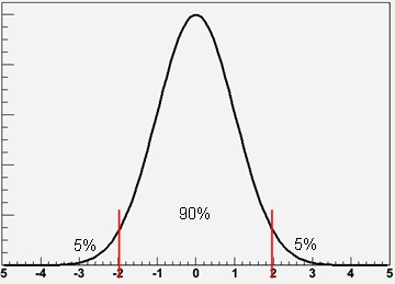
The graph shows the probable outcomes of your experiment if mu=0, but of course a similar Gaussian response function can be inferred for any other value: for a given mu you know what your experiment should find for x. Let us develop this standardized example: you have a measuring device which produces an estimate x of a quantity of unknown value mu. The error on the estimate x is Gaussian, and we choose as units of measurement for both x and mu the sigma of the Gaussian; or if you prefer, we assume that the sigma is exactly 1.0.
If you repeat the construction of the central 90% x intervals for all mu's, and you end up with a set of intervals, which "paint" an area of the "mu versus x" plot, and it might look like the figure below (taken from the original Feldman-Cousins paper of 1998). The intervals are seen to make up a confidence belt, which is the area delimited by the thick black lines (note the step at x=3 and the other features). This belt does not need any experimental measurement to be constructed: it rather uses information on the measuring apparatus and method used by the experimenter, and it tells us what conclusions we will be able to draw on the range of possible values of the parameter mu, depending on the estimate x we make of it. (Note, incidentally, that x and mu need not describe the same physical quantity: I might be measuring the temperature of a star by determining its peaking light wavelength, and the same construction can be made).
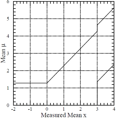
A few comments on how the belt is constructed in this plot: as you can see, here the physicist will quote an interval for mu if he finds x>3 (that is, if x is over three standard deviations away from zero); this is evident if you pick, say, x=3.5 and follow the vertical line at that value until you intercept an area of the belt. On the other hand, he will only quote a upper limit for x<3 (all the region from 0 to 3.28, say, is allowed if x=2); but if x becomes negative, he will refrain from quoting too small or null intervals for mu (as would be the case if he measured, say, x=-2, which would exclude all possible non-zero values of mu if the physicist were to obey the diagonal line), by quoting a upper limit at 1.28-sigma (a one-sided 90% interval) in that case.
Once you have a confidence belt, you can reverse the argument, and say: "I measured x=x0 in my real data, so now what are the values of mu compatible with that, at the confidence level I pre-defined in the construction of the belt ?". The answer is simple: it is the set of values where the confidence belt intersects the vertical line at x=x0. The mathematical proof of the fact that the vertical segments intercepted by the belt encompass the same fraction of the total probability as the horizontal segments we used to build the belt is simple but unfit for this post.
So the confidence belt gives your answer very simply: measure x and the belt will tell you where mu is; 90% of the time this information will be correct, because the coverage you required when you constructed your belt is 90%.
Then, what is flip-flopping again ?
Flip-flopping enters because you choose a value of x above which you decide to claim an observation of a non-null value of mu. If x>3, for instance, you are three standard deviations away from zero, so you may decide to use your data to measure mu, rather than to quote an upper limit; if x<3 on the other hand you keep a low profile (you do not want to "measure" mu if it turns out to be zero, because this would be embarassing; for instance, you do not want to say that the Higgs exists and that its production rate is mu, when the Higgs does not exist in fact, and the production rate is thus zero). So if x<3 you choose to rather quote an upper limit. (In the construction of the mystery figure I used x=4 instead, but the same arguments apply).
The construction of the belt will have to accommodate for this different treatment of the data depending on the outcome of the experiment: for values of x above 4, the quoting of a central interval rather than an upper limit forces the confidence intervals to be two-sided, with long-range effects on the coverage for different values of the unknown parameter mu.
It turns out that for a wide range of values of mu -specifically, from 2.36 all the way to 5.28- the coverage of the intervals is not 90%, but 85%. This is described by the central horizontal segment in the mystery plot I attached at the beginning of this article. Only for values of x larger than 5.64 will the nominal 90% coverage be reobtained. On the other hand, the feature of the belt for small and negative values of x creates "overcoverage" below x<1.28: that is because the construction of the belt implied that you avoid null intervals by "power-constraining" the limit: if you measure x<0, you act as if you had measured x=0, because you become not confident of your measurement, or because you want to avoid a very negative result for x to bring you to make very restrictive conclusions on mu.
The flip-flopping issue, with the resulting undercoverage in a wide region of possible outcomes for x, was pointed out by a groundbreaking article in 1998 by Gary Feldman and Robert Cousins. The article has received over 1100 citations in scientific publications this far. The authors of the paper re-discovered a principled method to overcome the trouble of the pure Neyman construction -i.e. the coverage issues, the flip-flopping defects, and the issue of null intervals. It is a sad fact that despite the wide use of the Feldman-Cousins approach to the limit-setting problem, in High-Energy physics the method is still not used very frequently. I hope we will change this situation at the LHC, but it will not be easy.


Comments