The Corfu Summer Institute is a well-established institution for higher education, run since the paleolithic by the inexhaustible George Zoupanos, the soul of the whole thing. Generations of physicists have been trained in doctoral schools and conferences there over the past few decades. Of course the beauty of the island, set in the Ionian sea and green from the top of its mountains to the blue sea below, has helped to keep the events there well-attended, and even during the pandemic the events have been run in person.

This year, besides other schools and workshops, a school in quantum gravity and astrophysics was organized by a group of theorists and experimentalists led by José Manuel Carmona (University of Zaragoza). They won a COST action grant from the European Commission, and one of their work packages involves the training of PhD students on the topics at the focus of their scientific program. I was thus delighted to accept their invitation to lecture about statistical methods for data analysis, as not only do I like this kind of dissemination activity (and I really recognize the need to train our PhD students on that topic), but I also love to pay random visits to Greek islands.

My visit was short - I arrived on Sunday and left on Wednesday - but intense, as I was able to squeeze in four full hours of lectures, and I gave online two more hours of tutorials (with root-based macros) this morning, upon my return to Padova. The lectures are not very different from those I give every year to PhD students in Padova, but the format of the school invited me to reorganize the material in a more coherent way; also, the organizers require lecturers to produce lecture notes, with the help of a couple of students each. So I'm happy that this time I will have a chance to produce a write-up of my explanations...

Here I will not be able to give you any summary of the six hours of lectures, but I do want to touch on a topic that is dear to my heart, the one of ancillary statistics. The reason I want to speak about this here is that it is a topic quite overlooked by textbooks in Statistics for data analysis, but it is one of fundamental relevance for interval estimation.

Ancillary statistics

Do you know what is an ancillary statistic? An ancillary statistic (ancillary to some other) is a function of the data which contains information on the precision of the inference you can make on some parameter based on the statistic you construct to estimate it, but no information on the parameter value itself. I'll go straight to a simple example before you try to wrap your head around the sentence above.

Imagine you want to estimate the location of a box distribution - one which has a density function which is uniformly equal to 1.0 in a unit interval, e.g. [0,1] or [pi, pi+1], and zero elsewhere. Such a distribution is obviously automatically normalized - i.e., it is a probability density function in its own right. The "location", call it μ, be understood to be the center of the distribution, so μ=0.5 for a [0,1] box, exempli gratia.

Now, you are given two data points drawn from the distribution: x1 and x2. You immediately realize that the best estimate of the center of the distribution is the mean of x1 and x2, i.e. 

<x> =(x1+x2)/2. 

In truth, if you said "mean", your understanding is liable to be flawed, but only virtually so. Indeed, the above expression is exactly the maximum-likelihood estimate (MLE) of the box center, if you have two observations. On the other hand, if you had more observations, you should not take their mean no more, but rather compute the midpoint of the most extreme pair of data -all other data points are sampled from a uniform density within the two most extreme ones, and contain no information whatsoever on the location! But this is a detail of academic interest in this specific example, so let us move on [I know precisely one example in HEP practice when this observation made a significant difference, which unfortunately the authors of the analysis did not realize... The Opera measurement of neutrino speeds!]

You also understand that the precision of that estimate depends on how lucky you were in drawing x1 and x2, for if the two numbers are far apart (i.e. their difference is close to 1) the box is constrained very precisely, while if x1 and x2 are very close to one another (i.e. their difference is close to 0) the box is ill-constrained, as it can be moved freely by almost a full unit to the left or to the right of the two observed values.

What this tells you is that there is, in fact, a function of the data which is sensitive to the precision of the location estimate, but has no information on the location itself. This function is indeed Δ=|x1-x2|, the distance of the two points. It is easy to prove that  bears no information on the location μ, and I will not bother unleashing derivatives here (but if you're curious: just obtain d(x1+x2)/d(x1-x2)=0 by the chain rule of differential calculus to show it). Instead, the uncertainty on the mean value (x1+x2)/2, computed as a maximum error, is equal to 1-Δ.

Now, if you are only concerned with the point estimate for the box location you need not worry at all about the fact that Δ is an ancillary statistic. But if you need to report a confidence interval of the estimate, Δ suddenly becomes an elephant in the room. Let me explain how the interval estimate could be cooked up in the classical way, which guarantees the property of coverage of the produced intervals.

Neyman's belt

The construction is called "Neyman's belt" and it is what allows you to report a confidence interval upon estimating a parameter, knowing that the interval (a random variable function of the data you collect) is drawn from an imaginary sample which possesses the property of coverage: 68.3% of the intervals in that set contain the unknown, true value of the quantity being estimated. 

Note that for a classical Statistician it is not true that any given interval on the parameter, even if cooked up with Neyman's construction, covers at 68.3% (the so-called "one-sigma interval"): it is the set of all possible intervals that enjoys the property, not any given interval! 

Now, for Neyman's construction: it all boils down (for the estimate of a one-dimensional parameter based on a one-dimensional observation - in our case the estimate of μ based on the average <x> of x1 and x2) to a three-step procedure (preceded by two preliminary steps!):

-1) Choose a confidence level for the intervals you are going to report. Let this be 0.683, the classic one-sigma interval. Also choose an "ordering principle": in our case, we will be interested with reporting central confidence intervals, so ones that exclude 15.85% of the probability density on each side.

0) Consider a graph where on the abscissa you have the average of x1 and x2, and on the ordinate the true, unknown value of the box center μ.

1) For every value of the unknown parameter μ, determine what is the probability density function that describes the distribution of the average you can observe, given that μ. This is written p(<x>|μ), where <x>= 0.5(x1+x2). In our case, as we plan to compute the estimate of the box location as the mean (or midpoint, if we know better and are sufficiently fussy) of two observations, that function is a triangular distribution of width 1, as it is easy to convince yourself by thinking at the two values as points in a square of unit side, and projecting their sum over the diagonal.

2) Determine the values of x corresponding to the 15.85% and the 84.15% percentiles of the distribution, x_low(μ) and x_up(μ) for every μ. These can be plotted as functions on the graph.

3) Now you have a "belt", that is the region contained within the two curves. Note that until now we have not yet performed the actual measurement of x1 and x2! The belt, in other words, exists once the measurement procedure (the decision to take two samples from the box distribution, and average them to get the estimate of the center) is defined, and (very importantly) once you have done also point -1, i.e. decided on a size of the confidence interval and an ordering prescription for how you select what points of the density functions to contain in the intervals.



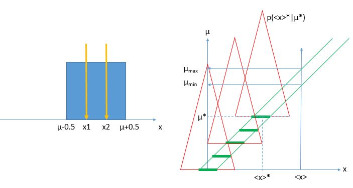
[Above: left, the box distribution and two measurements taken from it; right, the construction of the Neyman belt (area within the two green lines) given the density functions p(<x>|μ) (red triangles). The thick green segments highlight central intervals for different values of μ, covering 68.3% of the area of the triangles (if triangles have base of length 1.0 and height 2.0, as they should, the segments have an extension of 0.3415, because the area of triangles within that segment is equal to 0.683)]

Now, once you collect your data and determine <x>, you can go to the graph and draw a vertical line at that abscissa point. The vertical line will intercept the belt in some points (in a simple case, these will be two points; but note that the belt, in the most general case, might even be a non-connected set of areas of the plane, if the ordering principle is more complicated than the central one and/or if the parameter μ is not a continuous real-valued one). The union of all areas of the belt intercepted by the vertical line is the confidence interval you are after (in the figure, the interval [μ_min,μ_max]), and Jerzy Neyman himself guarantees you that it will belong to a confidence set - in other words, on average the intervals extracted this way cover at 68.3% the unknown location of the box!

Back to ancillarity - the elephant in the room

Ok, so where is the elephant in the room? Well, the construction you have just seen above is perfectly valid, but it is also a bit too general. In fact, the existence of a function of the data which bears no effect on the estimate, but is sensitive to the uncertainty of the estimate itself, forces us to revisit the Neyman belt construction.

Recall that the belt was constructed by considering the probability density function p(<x>|μ) for every μ, and every <x>. This is fine, but <x> is made up of two observations x1 and x2 in our case, and their being close or far apart changes the distribution of p(<x>|μ) of our particular measurement! In fact, consider what happens if |x1-x2| is equal to 0.9 - a lucky case. In those circumstances, the confidence belt should be very narrow, as we _know_ that the unknown μ cannot be more than 0.05 units away from <x> in each direction! On the other hand, if |x1-x2| equals 0.1, we have little constraining power - μ can have a lot more freedom to be located as far as 0.95 units away from the center of the measured interval. These two cases are "subspaces" of the sample space which was used for the Neyman construction. In Statistical parlance each of them is a "relevant subset" in the sense that each is the relevant subset of the sample space which we should consider if we get data with a Δ value of 0.9 or 0.1, respectively. 

Now, where does this lead us? To the observation that the Neyman belt is correct, but a bit too general. If we use the knowledge of what Δ turns out to be in our actual measurement - and we _can_ do it as Δ is independent on the estimated <x> ! (a very important condition, satisfied by the ancillarity of Δ) - then we may legitimately revise the Neyman belt by recomputing it using density functions which we may write p(<x>|μ,Δ), by "restricting the sample space" to the "relevant subset" given by all sets of x1, x2 measurements that fulfill Δ=|x1-x2| !

If we do that, our inference on the unknown box location will be much more precise, because we have been able to condition to the precision guaranteed by the data we actually obtained. Mind you - the uncertainty interval around our estimate of μ does not necessarily turn out to be smaller (that would violate some sort of a "free lunch theorem"), but it is still an interval that "covers" at the required confidence level, and it will more precisely track the actual situation and the uncertainty of our particular measurement. Now that you know how to compute a Neyman belt, try to do it by conditioning to different values of the ancillary statistic, and see what you get!

Ancillary statistics are not always there for you to pick, but they should be actively sought in any conceivable experiment, as their identification does improve the quality of your inference. I hope you will now think at your parameter estimation practice with different eyes!

And down here in this post, in a place where nobody will ever venture to read, I can safely hide the statement that I am deeply indebted to Bob Cousins for being first taught about relevant subsets during endless Statistics Commitee meetings and cafeteria discussions ;-)


---

Tommaso Dorigo (see his personal web page here) is an experimental particle physicist who works for the INFN and the University of Padova, and collaborates with the CMS experiment at the CERN LHC. He coordinates the MODE Collaboration, a group of physicists and computer scientists from eight institutions in Europe and the US who aim to enable end-to-end optimization of detector design with differentiable programming. Dorigo is an editor of the journals Reviews in Physics and Physics Open. In 2016 Dorigo published the book "Anomaly! Collider Physics and the Quest for New Phenomena at Fermilab", an insider view of the sociology of big particle physics experiments. You can get a copy of the book on Amazon, or contact him to get a free pdf copy if you have limited financial means.