I don't remember who said it, but there's a quote I like a lot: "If you torture them long enough, the data will confess to anything". What the author meant is of course that the manipulation of experimental data and the a posteriori use of hand-picked methods, approximations, and other ad-hoc choices allows you to demonstrate anything with them, from one hypothesis to the opposite one. Statistics, in other words, is a subtle science, which must be handled with care. It is a powerful tool in the hands of people with an agenda.
Yet I do not wish to discuss here how to lie with Statistics - this is a very well covered topic, and there are dozens of good books on the market that deal with its details. Rather, I mean good when I say I want to "squeeze more information" from the data. In fact, that is the research topic I have been working on as of late, for the purpose of improving the power of our statistical inference with LHC data. Those proton-proton collisions are a treasure of information, and we must ensure we obtain as much knowledge about subnuclear physics as we can from its study!
Squeezing more information from highly multi-dimensional data is the job of machine learning algorithms, such as neural networks or boosted decision trees, that are capable of creating powerful "summary statistics" from them, effectively operating a dimensionality reduction which enables the extraction of estimates of interesting parameters.
To make an example, if you want to know what is the rate of production of Higgs decays to b-quark pairs in data collected by a LHC detector, you may want to take the processed and reconstructed collision events - each of which comprise hundreds of different measurements - and extract a score per event in the [0,1] range which tells you how "Higgs to b-bbar"-like that event is. The machine learning algorithm will take care of assigning low values (close to 0) to background events, and high values (close to 1) to Higgs events. Armed with that summary, you can then observe the rate of events in the high-end tail of the distribution of scores.
The nuisance of nuisances
The job is harder than what is summarized above, because in addition to the unknown parameter you wish to extract, there are a number of other "nuisance parameters" that are capable of worsening your inference, as you do not know their exact value. For instance, if some of the hypotheses upon which your machine learning tool based its classification score is slightly off, the result on the parameter of interest is going to be biased. You have to then add a systematic uncertainty to your estimate, and that is quite a unwanted outcome!
To tame nuisance parameters, people have tried many different approaches. The one Pablo de Castro Manzano and I have put together, "INFERNO", promises to revolutionize the parameter estimates we do at the LHC when nuisance parameters are important, as the algorithm creates summary statistics that are optimally robust to the smearing effect of nuisance parameters, as the algorithm "learns" how to minimize the variance of the parameter estimate, after accounting for all nuisances! You can read about this method in a preprint we are submitting to Computer Physics Communications.
The other reason why I am writing today is that I have recently been discussing similar topics within a course I am giving to the Master students of Statistical Sciences in Padova, which is titled "Particle Physics: Foundations, Instruments, and Methods". It has been a tall order to cover the whole of experimental particle physics research in 64 hours of lectures, but I seem to be doing fine. In one lecture I discussed the topic of "ancillary statistics", and I wish to report here on what I taught my students during that lecture, as I believe it is stuff not known well enough within researchers.
It's ancillary, so pay attention
First of all, what is an ancillary statistic ? And, given its name, should we care at all about it ? Well, the answer to the second question is "most definitely!". An ancillary statistic is a function of your data which bears information on the precision of the parameter estimate you can obtain from the data, but NO information whatsoever on the parameter estimate itself. Since I often teach my students that a point estimate without a uncertainty is less informative than an uncertainty without the corresponding point estimate (thus thwarting any attempt to quote numbers without a +- sign on their right), you well understand that ancillary statistics get my attention. Interval estimation is a way more rich topic than parameter estimation if you ask me!
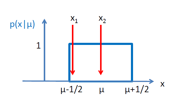
Let me make an example. Suppose your neighbor has a car that leaks oil from any point on its bottom part, and suppose you want to determine where along the road in front of his house the car was parked last night, based on the location of oil spots left on the ground. Your data are two spots left on the ground this time. We can model this problem by saying that there is a uniform "box" probability distribution for the location of the oil spots along an "x" axis which models the road. The width of the box is equal to the length of the car, and here we take it to have length of 1.0, for simplicity (or say we measure positions along x in car length units).
As I said, you get to measure the location of two oil spots on the ground. Now the question I have for you is, what is your a priori estimate of the uncertainty on the car's center (the center of the box distribution from which the oil spots are sampled)?
 An undergraduate student would reason that if the R.M.S. of each oil spot location is computed for a box distribution of width one, the answer is 1/sqrt(12), or approximately 0.29. A (biased, but let's not get stuck in details) of the uncertainty on the mean is then the RMS divided by sqrt(N), where N are the number of observations that get averaged out. One would find that the typical "1-sigma" interval has then a width of about 0.2. That number would be a rather coarse estimate of the interval around the mean which "covers" at 68.3% confidence level, because it has been derived assuming that the data are sampled from a Gaussian distribution, which they aren't.
Conditioning: more relevant inference
A more precise estimate, which is guaranteed to offer correct coverage in the classical sense, is the one you can obtain from Neyman's construction of confidence intervals. This, like the coarse estimate above, can (and is prescribed to) be obtained prior to observing your data. In that sense, it is unconditional of the actual sample you got (the two measurements x1 and x2 of the oil spot locations). With Neyman's construction your estimate for the uncertainty on the box location - which is of course equal to (x1+x2)/2, the mid-point of the two observed spots - would come up in the 0.25-0.3 range (forgive me for being imprecise - the calculation is easy but I have no wish to carry it out, nor is it important here).
What is important is that whatever estimate of the confidence interval width you get using the unconditional observation space is going to be rather imprecise, despite its guaranteed coverage. This is because the problem contains a subtlety that allows to identify an ancillary statistic: a function of x1,x2 which carries no information on the box location, but crucial information (actually, in this simple case all the information) on the precision of the inference.
Let us specify the data. Say the oil spots are at locations 0.9 and 1.1 along the x axis. You proceed to make an estimate of the location, and get 1.0, of course. With Neyman's construction your uncertainty would then be whatever number we found before the measurements, say 0.25. Now imagine instead that the oil spots were found at locations 0.501 and 1.499.
Again, your best estimate of the car location would be at 1.0. If you stuck with an interval estimate based on the unconditional space (i.e., prior to the actual data coming in), you would still attach to that point estimate an uncertainty of 0.25 or whatever Neyman told you. But... In this second case it is obvious that the car's position is known with extreme accuracy, not with a coarse 0.25 error! That's because the wide distance between the oil spots guarantees that the car could not have been parked anywhere but at 1.0, while in the first case it could be anywhere between 0.1 and 1.9.
What is the ancillary statistic in this problem? A moment of thought should suffice to convince you that it is
α=|x1-x2|,
the absolute value of the difference of the two locations. α carries no information on where the car is, but it automatically tells you that the 68.3% confidence interval on the average of x1-x2 is
+- σ = 0.5 * 0.683 * (1-α) !
 The British statistician Cox (no, not Brian the entertainer, David, see right) has made an even more striking example of the concept. Suppose you have to measure a weight, and have two scales available. The first has a precision of 1 gram, the second a precision of 10 grams.
You of course would like to use the more precise scale, but the measurement procedure dictates, for obscure reasons we are not here to discuss, the tossing of a coin. If the coin lands on heads you get to measure the weight with the more precise scale, if it lands on tails you have to use the less precise one.
Now let me ask you: what uncertainty do you predict you will have on the weight estimate? Prior to the experiment (which includes the coin toss) you have to consider both possibilities; your uncertainty estimate will be somewhere midway between 1 and 10 grams, say 5.5 grams. But now please go ahead. You get a heads! You get to measure your weight with the precise scale, and obtain a weight of 352 grams.
What uncertainty do you assign to that point estimate? You certainly would want to say it is +- 1 gram! But the procedure unconditional of the observation outcome forces you to still use 5.5 grams. The coin toss here is the ancillary statistic, which knows nothing about the weight, but everything about the uncertainty!
Ancillary statistics are not easy to find in more complex problems, but if you can find them, you can partition the observation space such that your inference may become much more powerful (as your confidence intervals are more appropriately sized up). So look for them in your data whenever you suspect that the precision of the parameter estimate may depend on the vagaries of the observations you may get!
---
Tommaso Dorigo is an experimental particle physicist who works for the INFN at the University of Padova, and collaborates with the CMS experiment at the CERN LHC. He coordinates the European network AMVA4NewPhysics as well as research in accelerator-based physics for INFN-Padova, and is an editor of the journal Reviews in Physics. In 2016 Dorigo published the book “Anomaly! Collider physics and the quest for new phenomena at Fermilab”. You can get a copy of the book on Amazon.