

The general problem
Imagine you are given a set of counts distributed in bins of a histogram. This could be, for instance, the age distribution of a set of people. You are asked to assign uncertainty bars to the counts: in other words, estimate a "one-sigma" interval for the relative rate of counts in each bin.
[I will make a divagation here, as it is an important thing to note. Attaching uncertainty bars to observed counts is something that statisticians never do, but we physicists insist in doing. In general, the observed number of counts falling in a bin is a datum that carries NO uncertainty; however, physicists like to visualize the datum (a black marker, typically) together with a vertical bar which represents the "one-standard-deviation" variability of the quantity that the datum itself estimates. So let it be like that this time.]
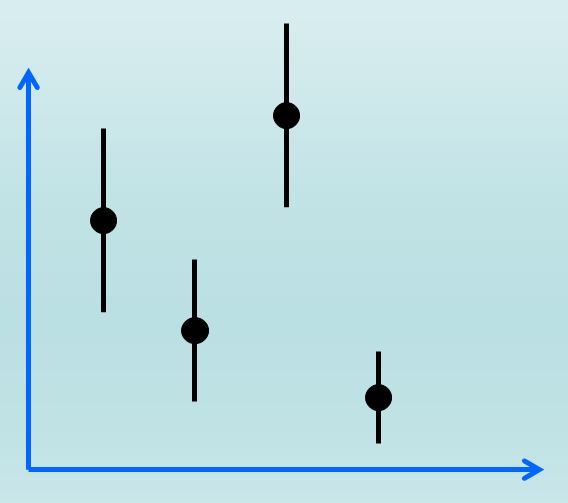
(Above: points with vertical bars representing their uncertainty.)
Now, if you take a random sample of people - say all those you meet in the street in a 20 minute walk - you would expect that the counts in each of the bins have "Poisson variates". This is because people of a specific age, say 35 years, cross your path at a certain rate (unknown but supposed fixed), during that time of the day and in that particular part of town. That defines numbers that have the property of being sampled from the Poisson distribution.
To explain better what all of that implies: if you one day observe N 35-year-olds, that N is your best estimate (in fact it is the uniformly-minimum-variance-unbiased estimate, and also the maximum-likelihood estimate) of the true, unknown rate μ of encounters with 35-year-olds in 20 minutes. Interestingly, due to the properties of the Poisson distribution N is also an estimate of the variance σ^2 of μ. This means that upon repeated walks when you entertain with measuring the true rate μ of 35-year-olds in 20' intervals, 68.3% of the time the observed number will have the property that N-sqrt(N) < μ < N+sqrt(N). This is what they call "coverage", baby.
So, ok you have a histogram of Poisson-distributed counts. Or is it ? That is the question I posed to myself in my specific problem.
I will tell you in a minute what my histogram was about, but here note that if your walk intersects many youngsters, your assumption of Poissonianity might be false, as youngsters like to hang around with people of their same age. The coverage of the above formula will then be screwed up for the bins of your age histogram encompassing ages from 8 to 20 years or so!
"Wait" - I can hear you interject - "what does the clustering of people with the same age have to do with the sampling properties of your bloody histogram?"
Well, everything! The fact that meeting a 14-year-old implies a higher probability of meeting another 14-year-old one second later entirely changes the statistical properties of my distribution. Let me prove that to you in the simple case in which people come in pairs of the same age.
In 20' I will e.g. see 2N 14-year-olds. The Poisson variable is N, with variance N. So, by using simple error propagation, we find that the observed count of 2N 14-year-olds has a variance equal to
The variance is twice as big as the one of 2N 14-year-olds who had arrived independent of one another!
So here is the problem, stated a bit better (and with some insight provided by the example above):
since the correlation between the appearance of entries in a specific bin of a histogram with the appearance of other entries (in that same bin, or in others) screws up the Poisson properties of the bin contents, how can we cook up a good test that can flag the non-Poissonianity?
The specific setup - Hemisphere Mixing
The problem as I stated above comes from a very specific physics analysis application. In practice, I have a way of obtaining, from a dataset of collision events, an artificial dataset that possesses the same properties. The technique, called "Hemisphere mixing", is a smart way to construct a proper background modeling for searches of new physics in data containing many hadronic jets. It has been discussed elsewhere and it would be too long to explain here, so let me give you only a taste of it.
In multijet events at the LHC, the topology is very complex. These events are hard to simulate with Monte Carlo programs, and since they have a large cross section, the CPU required is often prohibitive. One then resorts to data-driven methods to estimate their behavior, typically identifying "control samples" of data that are poor in the specific features one is interested in - like the presence of a signal of a new particle decay.
What the technique designed by the AMVA4NewPhysics network members does is to consider that each multi-jet event, despite its complexity, is the result of a 2-->2 reaction (two partons collide, two partons get kicked out) made complex by initial and final state radiation, pileup, multiple parton interactions of lower energy, etcetera. One may not easily identify a "thrust" axis which is the direction that the two final-state partons had, as the center-of-mass of the collision is not at rest in the laboratory frame; but one can do that in the plane transverse to the beams.
The transverse thrust axis identifies a plane orthogonal to it. The plane can be used to ideally "cut" the event in two halves. One may thus create, from an original dataset, a library of half-events (hemispheres). Then, events can be reconstituted by recombining these hemispheres in a proper way (I will save you the details). One thus gets an "artificial" dataset that models the background very well. The statistical properties of that sample are to be studied in detail... Thus the work that led to this article!
The test in practice
To test whether an observable feature X of the events might retain a correlation between its value x in the artificial event and its value x' in the original one, I will use a trick.
I take a subset of events from the original dataset and the corresponding events in the artificial dataset -their artificial replicas- to construct a histogram of the feature X. This means that there will be two entries per each original event in the subset of the original dataset: x, and the corresponding x' of its artificial replica. If x and x' are 100% correlated - like the two 14-year olds walking side by side - the resulting histogram will have bins exhibiting variances twice as big as what they should!
The test involves creating many subsets (by a suitable resampling technique), obtaining many histograms that should be equivalent to one another (i.e., in statistical terms, sampled from the same prior distribution). By computing the variance in each bin of these histograms, and comparing it with the mean of the contents in the same bin, one can cook up a very powerful test.
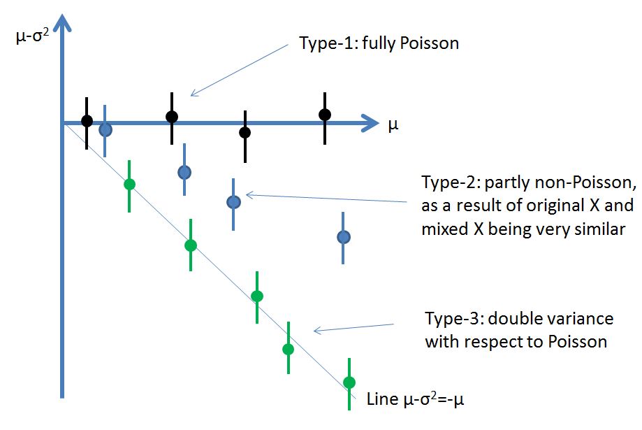
In fact what I did was to plot the average in a bin <N> minus the sample variance in that bin <s^2> as a function of <N>. For a set of Poisson histograms, I expect a set of points lining up at zero, as mean and variance should then be equal. For histograms where feature X in each event is correlated 100% in original and artificial data, I expect instead that the points line up along a downward line of -1 slope, as μ-σ^2=-μ!
The above test is quite powerful as it can detect very small non-Poisson nature in the distribution of the bin contents. Below is a graph showing that for five of the six tested features the blue points (the ones really under test) do bounce around zero, while for the sixth (bottom right) they exhibit a marked non-Poissonianity (indeed that variable was one I was expecting to be very correlated in original and artificial data). What is nice is that this way one can explicitly measure the true variance for any feature in the data!
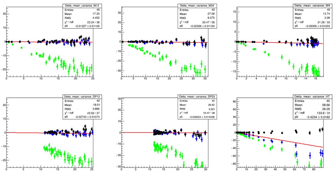
In the figure above, the green points show the behaviour of the variance in the bins of histograms constructed with the same feature repeated twice - as expected, the points line up with a -1 slope (the two histograms on the lower left and center have always more than 10 entries so there are no estimates at low N, but the behavior is the same). The black points instead show a cross-check that demonstrates what a real independent histogram, constructed from original data alone, would show. The red lines are fits to the sets of blue points under test.
Below is a simplified graph showing the three types of tested histograms and their expected behavior in the test plot I cooked up.
Now, if you take a random sample of people - say all those you meet in the street in a 20 minute walk - you would expect that the counts in each of the bins have "Poisson variates". This is because people of a specific age, say 35 years, cross your path at a certain rate (unknown but supposed fixed), during that time of the day and in that particular part of town. That defines numbers that have the property of being sampled from the Poisson distribution.
To explain better what all of that implies: if you one day observe N 35-year-olds, that N is your best estimate (in fact it is the uniformly-minimum-variance-unbiased estimate, and also the maximum-likelihood estimate) of the true, unknown rate μ of encounters with 35-year-olds in 20 minutes. Interestingly, due to the properties of the Poisson distribution N is also an estimate of the variance σ^2 of μ. This means that upon repeated walks when you entertain with measuring the true rate μ of 35-year-olds in 20' intervals, 68.3% of the time the observed number will have the property that N-sqrt(N) < μ < N+sqrt(N). This is what they call "coverage", baby.
So, ok you have a histogram of Poisson-distributed counts. Or is it ? That is the question I posed to myself in my specific problem.
I will tell you in a minute what my histogram was about, but here note that if your walk intersects many youngsters, your assumption of Poissonianity might be false, as youngsters like to hang around with people of their same age. The coverage of the above formula will then be screwed up for the bins of your age histogram encompassing ages from 8 to 20 years or so!
"Wait" - I can hear you interject - "what does the clustering of people with the same age have to do with the sampling properties of your bloody histogram?"
Well, everything! The fact that meeting a 14-year-old implies a higher probability of meeting another 14-year-old one second later entirely changes the statistical properties of my distribution. Let me prove that to you in the simple case in which people come in pairs of the same age.
In 20' I will e.g. see 2N 14-year-olds. The Poisson variable is N, with variance N. So, by using simple error propagation, we find that the observed count of 2N 14-year-olds has a variance equal to
The variance is twice as big as the one of 2N 14-year-olds who had arrived independent of one another!
So here is the problem, stated a bit better (and with some insight provided by the example above):
since the correlation between the appearance of entries in a specific bin of a histogram with the appearance of other entries (in that same bin, or in others) screws up the Poisson properties of the bin contents, how can we cook up a good test that can flag the non-Poissonianity?
The specific setup - Hemisphere Mixing
The problem as I stated above comes from a very specific physics analysis application. In practice, I have a way of obtaining, from a dataset of collision events, an artificial dataset that possesses the same properties. The technique, called "Hemisphere mixing", is a smart way to construct a proper background modeling for searches of new physics in data containing many hadronic jets. It has been discussed elsewhere and it would be too long to explain here, so let me give you only a taste of it.
In multijet events at the LHC, the topology is very complex. These events are hard to simulate with Monte Carlo programs, and since they have a large cross section, the CPU required is often prohibitive. One then resorts to data-driven methods to estimate their behavior, typically identifying "control samples" of data that are poor in the specific features one is interested in - like the presence of a signal of a new particle decay.
What the technique designed by the AMVA4NewPhysics network members does is to consider that each multi-jet event, despite its complexity, is the result of a 2-->2 reaction (two partons collide, two partons get kicked out) made complex by initial and final state radiation, pileup, multiple parton interactions of lower energy, etcetera. One may not easily identify a "thrust" axis which is the direction that the two final-state partons had, as the center-of-mass of the collision is not at rest in the laboratory frame; but one can do that in the plane transverse to the beams.
The transverse thrust axis identifies a plane orthogonal to it. The plane can be used to ideally "cut" the event in two halves. One may thus create, from an original dataset, a library of half-events (hemispheres). Then, events can be reconstituted by recombining these hemispheres in a proper way (I will save you the details). One thus gets an "artificial" dataset that models the background very well. The statistical properties of that sample are to be studied in detail... Thus the work that led to this article!
The test in practice
To test whether an observable feature X of the events might retain a correlation between its value x in the artificial event and its value x' in the original one, I will use a trick.
I take a subset of events from the original dataset and the corresponding events in the artificial dataset -their artificial replicas- to construct a histogram of the feature X. This means that there will be two entries per each original event in the subset of the original dataset: x, and the corresponding x' of its artificial replica. If x and x' are 100% correlated - like the two 14-year olds walking side by side - the resulting histogram will have bins exhibiting variances twice as big as what they should!
The test involves creating many subsets (by a suitable resampling technique), obtaining many histograms that should be equivalent to one another (i.e., in statistical terms, sampled from the same prior distribution). By computing the variance in each bin of these histograms, and comparing it with the mean of the contents in the same bin, one can cook up a very powerful test.
In fact what I did was to plot the average in a bin <N> minus the sample variance in that bin <s^2> as a function of <N>. For a set of Poisson histograms, I expect a set of points lining up at zero, as mean and variance should then be equal. For histograms where feature X in each event is correlated 100% in original and artificial data, I expect instead that the points line up along a downward line of -1 slope, as μ-σ^2=-μ!
The above test is quite powerful as it can detect very small non-Poisson nature in the distribution of the bin contents. Below is a graph showing that for five of the six tested features the blue points (the ones really under test) do bounce around zero, while for the sixth (bottom right) they exhibit a marked non-Poissonianity (indeed that variable was one I was expecting to be very correlated in original and artificial data). What is nice is that this way one can explicitly measure the true variance for any feature in the data!
In the figure above, the green points show the behaviour of the variance in the bins of histograms constructed with the same feature repeated twice - as expected, the points line up with a -1 slope (the two histograms on the lower left and center have always more than 10 entries so there are no estimates at low N, but the behavior is the same). The black points instead show a cross-check that demonstrates what a real independent histogram, constructed from original data alone, would show. The red lines are fits to the sets of blue points under test.
Below is a simplified graph showing the three types of tested histograms and their expected behavior in the test plot I cooked up.
----
Tommaso Dorigo is an experimental particle physicist, who works for the INFN at the University of Padova, and collaborates with the CMS experiment at the CERN LHC. He coordinates the European network AMVA4NewPhysics as well as research in accelerator-based physics for INFN-Padova, and is an editor of the journal Reviews in Physics. In 2016 Dorigo published the book “Anomaly! Collider physics and the quest for new phenomena at Fermilab”. You can purchase a copy of the book by clicking on the book cover in the column on the right.


Comments