

Before I explain what I mean with the above, I will mention that the reason for this post was originally to advertise a seminar I gave on June 15th at CERN. In it, I discussed two recent articles I published. In both cases I used old-fashioned multivariate analysis tools to solve problems that are today usually approached with deep neural networks: multivariate regression, and anomaly detection.
The title and abstract of the seminar are as in the screenshot below:

While the two articles focus on very different problems, I found it useful to discuss both because the computing tools I used to solve the problems are ones that have been around for many decades; yet I was able to retrofit them with the engine that makes neural networks work wonders.
Indeed, the possibility to compute the derivative of some utility function as a function of the parameters of a problem enables the investigation of the parameter space with a procedure called "gradient descent", and this is not something you need a neural network to use. Suppose you are looking for a dead rat in your basement. The stench increases as you get closer, so you know how to find the corpse: you just walk in the direction of steepest gradient of smell - where the intensity is growing the largest per step you take. You do not need a neural network to put together this algorithm!
The other important ingredient of neural networks and similar systems, which allows the utility function to become a smooth function of the parameters of the problem, easing the convergence to its extremum, is overparametrization. If you give your system the flexibility to be described by a large number of variables, you make life easier to your gradient descent algorithm.
Two multivariate problems - 1: Supervised Regression with a kNN
To prove that old-school approaches can reach performances similar to those of neural networks if you endow them with gradient descent and overparametrization, in the seminar I discussed the task of regressing the energy of very high-energy muons in a fine-grained calorimeter, something that was thought impossible until recently. Nowadays, deep convolutional neural network models can make sense of even very sparse information, such as the footprint those particles leave when they traverse dense materials. In a recent article we showed how this was possible, but then also tried to obtain similar results with a k-nearest neighbor approach. Results are very interesting, because to achieve a comparable performance we had to develop an overparametrized model and train a total of 66 million parameters!
If you do not know what a k-nearest neighbor algorithm is, I can explain it with the graph below. Suppose you need to estimate the temperature in Roscommon county from the data shown here. You could take the michigan state average of 56 degrees as a starter, but then you could reason that it would be more accurate to look for counties closer to the target. So you come up with the idea of the closest neighbor, which has a temperature of 55 degrees. That is kNN with k=1.
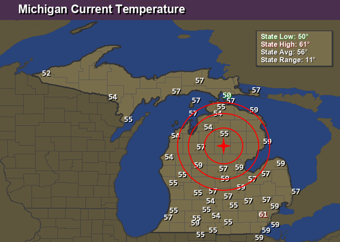
However, the single measurement in that closest neighbor has a high variance, because there is some variability in the temperature of any given measurement. So you can take the temperature of the 5 closest counties with reported data, and average them out. That is a kNN regression result with k=5. It will have smaller variance than the estimate with k=1, but in general it may have some bias, as you got to average temperatures of places that were a bit further away from the target.
In the cited article I applied a rather more complex procedure to estimate the energy of muons, but the core idea is the same of the kNN algorithm. In order to improve it, I assigned to every data point (like the temperatures in the graph) a bias and a weight. The bias is a random variation of the temperature, the weight a multiplier of that temperature reading in any average. When you average a few temperatures, if there are biases and weights you need to add all biases of the k neighbors, and add the sum to the weighted average of the temperatures. This means having introduced two extra parameters in the problem per each temperature reading.
Now you can try the procedure on some data of which you know the real temperature, and compute some measure of how far off your estimates are. This difference (your "loss function") is a function of weights and biases: now you can take the derivative of the difference with respect to all parameters, and modify parameters to improve its value.
While the above may look simple, it is tricky to do when you end up having 66 million parameters in your final algorithm. That is because the muon energy problem involved using several tens of variables in the determination of the distance -which determines who is close to whom- and I exploited that by creating many different averages, each constructed in subspaces of the variables determining the distance. If you want more detail, read the article...
The bottomline is shown in the graph below, where different curves describe the performance of different regressors in the task of measuring the energy of muons, as a function of muon energy. Here the lowest you are the better you are doing, because the vertical axis is the average error you commit in your estimate. Since the most important part of the muon energy spectrum is the one at very high energy (to the right in the graph), you see that the developed kNN algorithm (in black) performs similarly to neural networks and xgboost.
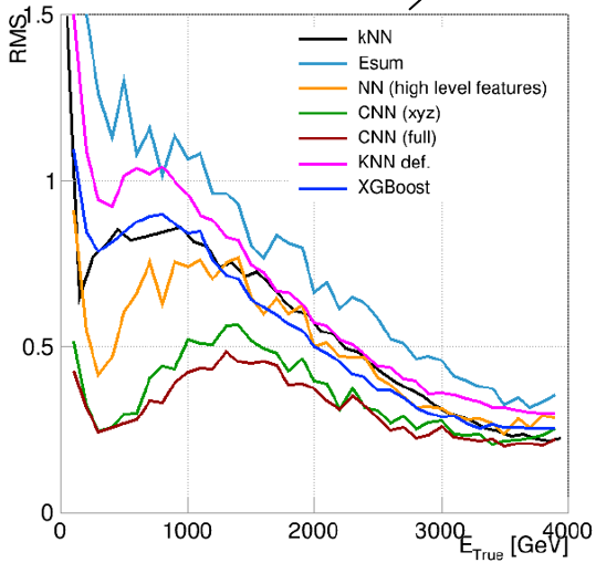
In the graph are also shown the results of the convolutional neural networks I mentioned earlier, but those should not be compared to the kNN because they could access full-granularity information on the calorimeter readouts, which the kNN was not given.
What the above shows is that you can use an old-school statistical learning tool and get performance comparable to that of today's neural networks. The catch, though, is the CPU requirements: the kNN models took literally a few weeks to run on a pool of 80 CPUs, while a NN can spew out that result in a couple of hours...
A Unsupervised Learning Problem: Finding Anomalies
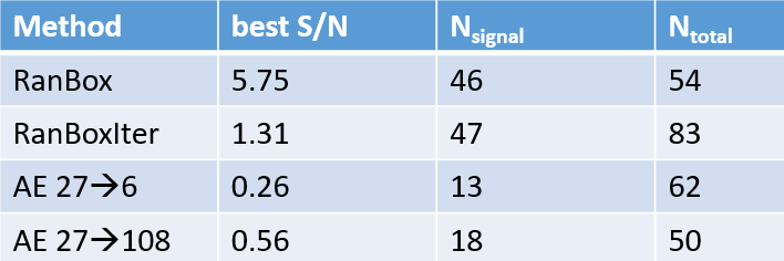
The second study I discussed in my seminar was the detection of small overdensities in a high-dimensional feature space. The algorithm I developed, called RanBox, does a search in the copula space... I discussed RanBox in a previous post here some time ago, so I will not repeat the whole story here, but the bottomline can be summarized by the table below.
In the table you see a bunch of numbers relative to four different methods to identify a small signal in a large dataset. RanBox and RanBoxIter are two versions of the algorithm I created to do this kind of "anomaly detection", while the other two lines refer to autoencoders, which are a special kind of neural network which can be used for the same unsupervised task. What matters here is that on the considered problem the autoencoders obtained less good signal identification than the two versions of RanBox - the column labeled "best S/N" represent the signal to noise ratio of the identified regions.
Mind you, you should never be satisfied with a single comparison of two methods for hypothesis testing or goodness or fit, like those above, as the performance usually depends on the particularities of the problem at hand. One should benchmark different algorithms on a number of different use cases in order to be able to say which works best. What the table above shows, however, is that an old-school algorithm based on square cuts in a multi-dimensional space can achieve good performances on very difficult multivariate problems, challenging neural networks - if you endow it with gradient descent functionality.
---
Tommaso Dorigo (see his personal web page here) is an experimental particle physicist who works for the INFN and the University of Padova, and collaborates with the CMS experiment at the CERN LHC. He coordinates the MODE Collaboration, a group of physicists and computer scientists from eight institutions in Europe and the US who aim to enable end-to-end optimization of detector design with differentiable programming. Dorigo is an editor of the journals Reviews in Physics and Physics Open. In 2016 Dorigo published the book "Anomaly! Collider Physics and the Quest for New Phenomena at Fermilab", an insider view of the sociology of big particle physics experiments. You can get a copy of the book on Amazon, or contact him to get a free pdf copy if you have limited financial means.


Comments