As silly as it may look, I am going to start this post by publishing for the third time in a row the same figure. That is because I want to keep the promise I made earlier that I would explain in terms as simple as possible (although not simpler) the details hidden behind the coloured curves and functions pictured there. I will also take this chance to come down a little from the level of technicality of the recent posts: after all, this blog is supposedly for everybody, and not just for Ph.D. students and recipients.

The figure above, a few of whose "secrets" I wish to unveil in the discussion below, shows the dependence of the as-of-yet unknown mass of the Higgs boson on W boson and top quark masses. This is a particular version of your generic "W mass versus top mass" plot (let us call it MW-MT in the following), actually: it is the one which uses as a measurement ellipse one constructed with the top quark mass taken as the one computed from the running top mass, an exercise performed recently in this paper, which I summarized in the former post.

Our goal for today will be to ignore the green area, which describes Supersymmetric model,s and just to grasp the reason for the logarithmic dependence of Higgs mass on top and W masses -the growing from 114 to 400 GeV of the Higgs boson mass as you move ever so slightly from the top to the bottom boundary of the red area-, and the parabolic shape of iso-Higgs-mass curves which delimitate it. This will take us deep in the details of quantum corrections to Standard Model observable quantities. Before we discuss those functional dependencies, at least a quick-and-dirty introduction is necessary.

Introduction: gauge symmetry and lagrangian functions

The Standard Model of particle physics is an amazingly elegant theoretical construction, which assumes a few crucial principles as its basis -among them quantum mechanics and local gauge symmetry-, and a few particles as its building blocks. Then, once you specify the blueprint, in the form of a well-defined group structure defining the forces these particles feel, and the resulting Lagrangian function, a marvelous complexity arises.

Already feeling uneasy about the few jargon terms in the previous sentence ? Worry not. Here are a couple of explanations.

The term "Lagrangian function" should not trouble you too much. A Lagrangian is just a function which enshrines the energy balance of the physical system we study. By specifying in it the various contributions to the total potential and kinetic energy of the bodies contained in the system, we can derive the laws of motion which govern the behaviour of those bodies. In other words, if we know how to write a Lagrangian function for the system, the rest of the work to predict the future evolution of the system is "just" a technicality.

The most complicated thing to define is "local gauge symmetry", a symmetry of the Lagrangian function. The mathematical expression of particles in quantum field theory includes an arbitrary complex phase, and the system has gauge symmetry if by changing the phase of these particle "fields" the Lagrangian, and consequently the equations of motion of the system, remains unchanged. Quantum fields describing particles are written as complex functions: these have a modulo and a phase, like vectors in a plane. Imagine rotating all vectors in a plane by the same angle, and you are visualizing a global gauge transformation.

Now, global gauge symmetry of a system is something nobody would object -a global complex phase is never an observable quantity anyway, and we all expect that the physical properties of a system do not change if we vary the phase of all fields. Moreover, one can prove that it is a highly desirable feature of the theory to be globally gauge invariant: if we consider electrodynamics, for instance, we can prove that global gauge symmetry of the Lagrangian ensures that electric charge is conserved. Imagine being a theorist who wants to find the laws of quantum electrodynamics, and comes up with a wonderful equation, which however allows net amounts of electric charge to be created at will from any point of space. Would you uncork your best bottle to celebrate ? No, you would begrudgingly go back to the blackboard!

A local gauge symmetry is much less trivial than a global one, and apparently it constitutes an eccentric request on the Lagrangian: the locality of the gauge symmetry implies that we can freely change the phase of all fields arbitrarily in different ways at different points of space without affecting the physics. Promoting to "local" a gauge symmetry is a crucial step in the path of constructing a particle theory, and the Standard Model has it among its foundations.

The reason for enforcing local gauge invariance to our Lagrangian was fully digested by particle theorists in the seventies, when it was conclusively proven in a giant achievement by 't Hooft that theories endowed with that properties are renormalizable. Just as much as non-local ones, local gauge invariant theories do describe physical processes which, if computed, contain infinite quantities; however, the infinities they generate can be eliminated by a redefinition of a finite number of arbitrary parameters. In quantum electrodynamics, for instance, one redefines the electron charge as a "renormalized charge", and the theory becomes capable of producing finite results: it therefore becomes a usable tool to compute and predict the measured value of observable quantities.

The Standard Model and virtual particle exchanges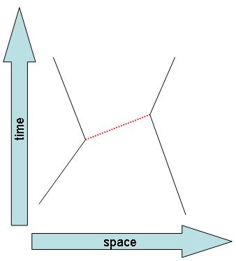

In the Standard Model, the interaction between matter fields (which are fermions: particles of half-integer spin) is described by the exchange of vector bosons. The picture is easy to draw: a fermion moving in space-time can be drawn in a plane as the left black line in the figure on the right, where we take time to flow on the vertical axis and space on the horizontal one. A boson emission by the fermion can be drawn as a bosonic line departing from the fermion at one well-defined space-time point, as shown by the dashed red line. Then, a second fermion can "absorb" the boson at a different space-time point, as described by the the black line on the right. As a result, the two fermions "feel" each other: they interact by exchanging the messenger, a vector boson. With not too complicated calculations it is possible to estimate the effect of this exchange, and compute measurable quantities, such as the scattering angle of the two fermions, their final energy, and so on.

Unfortunately, the above description is clean and simple, but we must realize two things: first, that the boson being exchanged is a virtual particle, and second, that our picture is incomplete. The boson is virtual because it is not an "asymptotic state", i.e., it is not a particle which at the end of the day is still part of the cast in the comedy we are enacting here: it made its apparition on the scene for a vanishingly small instant of time. And the picture is incomplete, because we only exemplified the interaction by discussing a single boson being exchanged; but in the subatomic world, there is no such limit. The interaction between the two fermions is the result of a force field rather than a single boson being emitted and absorbed: if we had more patience, we would have drawn more virtual actors in the figure, as below.

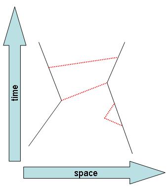
Note that it is entirely possible for a fermion line to emit, and then reabsorb, the same boson, as the lower-right fermion line does in the graph above. We can continue adding lines to the skeleton diagram, as in the third graph below.

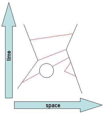
Above, you can see that not just bosons can be virtual: a boson can materialize a virtual fermion-antifermion line -the black circle- for a short instant of time. The asymptotic states described in the diagram do not change due to the inclusion of an arbitrary number of such virtual particle emissions and absorptions: at the beginning and at the end we just have the two real fermions, which scatter off one another; however, their kinematics is indeed affected by the higher-order corrections due to multiple exchanges.

The important thing to point out is that any time we add a virtual particle line in the picture and go back to the blackboard to compute the resulting effect on the measurable quantity we are trying to estimate, we are making our approximation of the real physics better; yet it remains an approximated view of what really happens. Now, quantum field theory allows to compute physical, measurable quantities out of these virtual diagrams. It turns out that the "higher-order corrections" to the value of the physical quantities, which result from accounting for more and more virtual exchanges, are smaller and smaller: the theory has the extremely valuable property of being perturbatively computable. This means that one can happily stop the calculation at a given order -i.e., by accounting for all diagrams which include a given number of virtual particle emissions-, in the certainty that the result represents a better approximation of the real value than the result obtained at a lower order.

Quantum corrections to heavy particle propagators

After the above introduction, I wish to show and comment a couple of diagrams which are crucial for the thrice-posted picture above. They describe the propagation in space-time of the W boson and the top quark. These two particles, together with the Z boson, are the three heaviest known elementary particles, and by virtue of their large mass, their coupling to the Higgs boson is largest. The Higgs boson, in fact, "feels" the mass of elementary particles, and it influences them with an intensity proportional to the particle mass squared. Because of that, by studying the phenomenology of W and Z bosons and top quarks, we gather information on the Higgs boson itself.

As far as the Z boson is concerned, its phenomenology has been studied by the four LEP experiments at CERN in the nineties. By using the amassed information on electroweak interactions involving Z bosons, it is indeed possible to extract a likely value for the mass of the Higgs. This is typically shown as an oblong, odd-shaped ellipsoidal area (labeled "LEP I and SLD") in plots like the one on the left, which demonstrates how not just the Higgs mass, but also the top quark and the W boson masses are indirectly determined by the LEP electroweak parameters. In the version of the MW-MT plot shown at the beginning of this post there is no such information, because it has become outdated -direct determinations of top and W masses are more precise; you can see it by comparing the blue ellipse -direct 2008 measurements of W and top masses- to the red one.

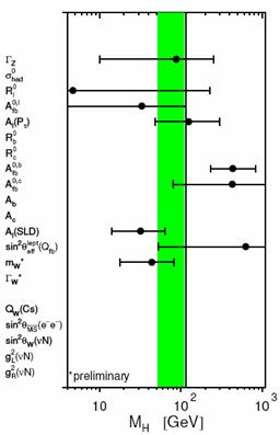The figure shown on the right here is also useful at this point. It demonstrates that there are a dozen different observable quantities measured by the glorious LEP experiments in electron-positron collisions at the mass of the Z boson, which can individually be used to infer the Higgs boson mass. Sure, they are imprecise, but together they do provide a powerful input. For each observable quantity, listed on the left as a column, a different Higgs mass bound can be obtained by comparing theory and measurement. These are shown as points with error bars; the green band shows instead the average value of the many determinations.

Anyway, let us forget about the Z here, and concentrate on the top and W masses, which are the ones that present-day experiments are trying to measure as precisely as possible. They, too, are influenced by the Higgs boson, and so they give independent additional information on the latter's mass.

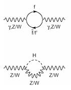The graphs on the left show examples of the quantum corrections that a heavy particle receives in its propagation, due to its coupling to the Higgs field. Above, a vector boson "fluctuates" into a fermion-antifermion pair (the circular "bubble") for a vanishingly small instant of time; below, a boson emits, and then reabsorbs, a virtual Higgs boson (the hatched line labeled "H"). I should note that these represent just one class of the possible virtual correction diagrams; I have no ambition to be precise in this article, and much less so exhaustive. However, I think you understood that these diagrams represent processes that, although "virtual", need to be accounted one way or another, in order to provide a theory which yields meaningful results from its calculations. 

Quantum corrections nail down the Higgs mass

So, there are heaps of graphs like the ones above which one may draw, and then compute. Their global effect causes a modification of one of the master formulas of the Standard Model: the one connecting the W and Z boson masses through the cosine of the so-called "Weinberg angle"  (paying tribute to one of the fathers of the Standard Model of electroweak interactions, Steven Weinberg). Knowing that each formula I post halves the number of my readers, I afford myself only two formulas today. Here is the first:

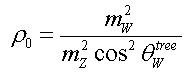
As you can see, the ratio between W and Z masses squared, modulated by the cosine of the Weinberg angle, is called "rho zero". Rho, at "tree level" -i.e. omitting quantum corrections- is equal to one in the SM. Quantum corrections such as those pictured in the figures shown above modify the value of rho. If one calculates the variation, one comes up with something like this, our second formula for today:

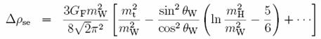
Now, if you belong to the 25% of readers who survived these two mathematical abuses, please forget the complications in the latter expression and the odd coefficients, and focus on one simple fact: the formula for the variation of rho from unity contains the squared W and top masses (labeled and , duh), and the logarithm of the Higgs mass squared (guess its symbol). Now, rho can be measured, because we do measure W and Z masses, as well as the Weinberg angle, the latter in a number of ways. So here is the key: by measuring electroweak parameters and masses of bosons and top quark, we can insert them in the formula above, invert it solving for mH, and extract an estimate for the logarithm of the Higgs mass!

(One word of caution: the formula above is not the whole story as far as the variation of the rho parameter is concerned; it only describes the variation due to "self-energy" diagrams. Again, my purpose here is to be didactic and not exhaustive).

There you have it. If you look again at the MW-MT plot, you can appreciate how indeed the variation of Higgs mass caused by a downward shift of the W mass, or -much less dramatically- by a upward shift of the top mass, is very fast: it is the consequence of the inversion of the formula to explicitate the Higgs mass. By the same token, you can now understand why the figure shown above, where different determinations of the Higgs mass using different electroweak observables are displayed, is made with a logarithmic horizontal axis.

I think you will forgive me now, dear readers, if I stop this post here before it becomes too long to be fruitful. There would be a whole lot more to say about this topic, but I reserve the right to verify whether this post was indeed read by a sufficient number of readers, and the amount of time they spent here. I do not mind a small audience, but the effort must be adequate to the return...