

In the course of the software development, I ran into a simple but still interesting statistical issue I had not paid attention to until now. So I thought I could share it with you here.
The running average is a very well known statistic to display time-series data; it is e.g. ubiquitously employed in finance applications, such as to show the long-term or even mid-term behavior of stocks. The concept is pretty simple: if you have to graph the time variation of a quantity you are monitoring, and this quantity is subjected to fluctuations that make every single determination noisy, you can smooth it out by taking the average of the last N measurements.
Consider, e.g., the series of measurements of a quantity X: x1,x2,x3,x4,x5,x6,x7,x8,x9,x10, taken at regular intervals of 1 day on ten consecutive days. From day three on you could report RA3 = (x1+x2+x3)/3 as your best guess of the value of X. On the next day you would then discard x1 and introduce the new measurement x4: RA4 = (x2+x3+x4)/3. And so on. By discarding the "long gone" x1 and including the fresh new estimate x4, the new RA4 is more precisely tracking the current value of X.
Note that, due to the fact that the true value of X is not guaranteed to have been constant in the last three days, there is something not completely correct going on. And indeed, this procedure will introduce bias, as you will not be measuring the value of the quantity at the last time step but rather a linear combination of the recent N values. So, e.g., if the true value is growing, a running average of its measurements will be biased negatively, as less recent, lower-expectation-value measurements will "pull it down".
Regardless, if the variations are not large and measurements are frequent, the running average is a robust display tool and also a predictive statistic. Note how this is just another example of the very common topic named "bias versus variance tradeoff" which one finds in many statistical applications: we accept some bias in an estimator to reduce its variance (the spread of measurements due to noise is reduced).
Now, the above is in any Statistics 101 coursebook, so why am I wasting your valuable time here? Because there can be interesting situations in the corners of the domain of application. It is again a common thing in Statistics that procedures that have general validity exhibit interesting behaviour in the presence of constraints or other special conditions or pockets of the phase space. Let us discuss in fact what happens if you know for a fact that the quantity you are estimating is monotonously growing with time.
One thing you could think of doing, if you wanted to graph the monotonously-growing "envelope" of the points (a curve of ever-growing estimate, which shares the monotonicity with the true value) is to apply the following algorithm:
1) compute the RA of the first N consecutive data points (e.g., N=3 as above).
2) every time you collect a new point, recompute the RA of the last N. If the new RA is higher than the previous one, accept the new measurement - as you wanted, this will produce a growing curve.
3) If, instead, after collecting a new point the new N-point RA steps below the previous best one, take the average of all points from the previous best to the last point, _including_ the previous best (which will thus decrease a bit) - i.e., update the previous best to conform to the newly found best RA. Then compare the new RA with the point preceding the previous best (the last non updated one), and if it is still lower than it, include it in a new RA that further decreases. Iterate until no previous RA exhibits the unwanted behavior of being higher than the RA of the last points.
The above procedure strictly obeys the monotonicity you want. But if you use it to plot the behaviour of slowly-growing quantities, you encounter a problem: the resulting graphs "flattens out", failing to capture any slow growth. The reason is that you are effectively operating a multiple testing procedure: you allow your RA to inquire multiple times about the growth from the last upward step, by including more and more points that have a chance to fluctuate down. By asymmetrically "pushing down" the average when it goes down, and not raising it when it goes up, you create a unwanted flattening.
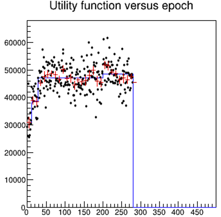
["Is it growing?" The black points are the "time-series" data; the red crosses are 10-point averages (no running); the blue histogram is the result of the recipe discussed in the text above.]
There are many ways to fix this unwanted feature. One involves dropping the iterative point 3) in the procedure above, and bumping up the highest-so-far RA only if the new estimate is significantly higher - when the significance is itself a function of the precision of the average of all the measurements from the previous best estimate. Since, e.g., the RA of three points has a considerably higher uncertainty than the RA of ten points (about 1.7 times smaller), you can be more confident that the latter signals a real variation in the value of the estimator. So point 2) above can be modified as follows:
2') every time you collect a new point, recompute the RA of all points from the one where the current maximum was first reached, _and_ estimate the uncertainty sigma_RA of this new RA. Accept that there has been an increase only if the new RA fulfils a significance criterion, e.g. new_RA - k* sigma_RA > old_best_RA (with k equal to 1 or 2, e.g); otherwise, keep the highest_so_far RA evaluation equal to the previous one (flat curve).
3') If instead new_RA + k*sigma_RA<old_best_RA, add the previous RA to the pool and get the average of all points, updating the curve as before. In that case, you need to iteratively check all previous RA's in turn, to avoid breaking the monotonicity.
The above amendment would seem to fix the procedure: surely, we are now confident that we are not taking action following a downward fluke?! In fact, it doesn't: because we are testing the condition multiple times as we go, we again give increasing chances to downward flukes to push the RA down.
How to fix it? We can make k vary with the number of measurements, to force the update-the-previous-highest-RA procedure to be applied only in more and more rare circumstances. One such update law for k that works is k = sqrt(log(N)) where N are the averaged points from the old maximum. One can fiddle with this and see that indeed it works fine, but I think there is no perfect solution to this problem. This is because the question is ill-posed: we pretend to be able to find a function that approximates the behaviour of the growing X, when we have no clue of what mathematical form that function has - we only know it is monotonous.
Any recipe, at this point, may have its merits, but no recipe can in general be better than another. This is another lesson in Statistics: there is no universal recipe for hypothesis testing - the power of any particular statistic will depend on the details of the alternative hypothesis you are testing (in this case, you can think of the alternative hypothesis as "the function is growing", and the null as "the function is flat).
The above realization, I think, is a relief: I can stop searching, and jolly well settle on something I like, without feeling I've not studied the matter deeply enough!


Comments