

These days I am in Paris, for a short vacation - for once, I am following my wife in a work trip; she performs at the grand Halle at la Villette (she is a soprano singer), and I exploit the occasion to have some pleasant time in one of the cities I like the most.
This morning I took the metro to go downtown, and found myself standing up in a wagon full of people. When my eyes wandered to the pavement, I saw that the plastic sheet had circular bumps, presumably reducing the chance of slips. And the pattern immediately reminded me of the Monte Carlo method, as it betrayed the effect of physical sampling of the ground by the passengers' feet:

As you can see, the area on the pavement close to the pole used by passengers to cling to during the rides shows a much better defined pattern of circular bumps than the area around it. The obvious reason for this is that people walk more often away from the pole than close to it, and over time this has built up to produce a disuniform wear of the bumps. What is not obvious, and is interesting to an enthusiast of the Monte Carlo method such as I am, would be to predict the profile of the wear as a function of the distance from the pole. That is something that can be studied numerically, as I will try to explain.
Ulam and the Monte Carlo method
The Monte Carlo method is credited to the nuclear physicist Stanislaw Ulam, who worked at the Manhattan project (but as far as I remember is not featured in Nolan's excellent movie about Oppenheimer). Below is a picture of Ulam I grabbed from his Wikipedia page. He sports the look of the guy who can peek inside your brain's probability distribution functions, and is shown with his laptop bag under his arm. Like me, he never parted from his laptop, and he used it to make wonderful calculations of complex probabilities for nuclear reactions. (Yo, I am kidding, yes).
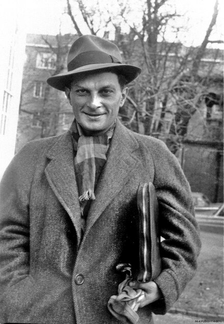
(Picture credit: Wikipedia)
In a nutshell, the Monte Carlo method consists in randomly sampling the space of possible outcomes of a process, to assess the odds of each. This usually returns a map of probabilities, which can be used as an input to calculations that cannot be performed by analytical means.
Let us say, e.g., that you wish to know the frequency at which buses 25 and 26 pass in front of your home. You could look this up on the web page of the bus company, of course, but let's pretend there is no published timetable. What you can do is to do a "Monte Carlo sampling" of bus appearances: you peek at random intervals out of the window, noting each time if any of the two buses is in sight, staring for 10 seconds each time. After you do it 360 times, e.g., you will have "covered" a total time of one hour, and the number of sightings of each bus will be a good estimate of its hourly frequency, averaged over the period over which you have distributed your peeking.
Note that the buses could have different frequency at different times of the day, in which case the Monte Carlo sampling you did would be unsuitable to get the fine structure of the timetable. But otherwise, the method is more robust to systematic effects than the alternative of staring out of the window for one hour in a row: in the latter case, you risk picking a time when there is a hyatus in the bus frequency, or when particularly bad traffic conditions alter the frequencies you are after; the random sampling "covers" more ground in a stochastic way. The averaging it performs is its strong point, in fact.
If your problem is the bus schedule you could well think that Ulam's concoction is not so useful. But the method is instead extremely powerful, especially today when even the lowest priced PC packs enough CPU power to perform billions of calculations in a jiff. The real power of the method, however, is realized in particular when the space of possible outcomes is so high-dimensional, and/or the process you are studying is so complicated, that there is no means to probe it with analytical means. Which does sound like particle physics, doesn't it? In fact, the method was developed specifically to assess the odds of nuclear reactions, which involve stochastic processes of very high complexity. Ever since Ulam, Monte Carlo -based calculations have been used in a wide range of applications.
A physics example
To give you a bit more perspective, let me summarize for you a particle physics example of the Monte Carlo method at work in the calculation of the probability that we observe a Higgs boson in the CMS detector at the CERN Large Hadron Collider.
The Higgs boson is produced with a very small probability in proton-proton collisions. For any given collision, calculating the production rate involves summing up the contribution of a very large number of different physical reactions, each of which is calculable by analytical means. It is complicated, because each term depends on two unknown quantities: the fraction of their parent proton energy, x, that is carried by each of the partons (quarks or gluons) that hit each other. x is a number between 0 and 1, and the larger it is, the more probable (according to some complicated analytical function that theorists can cook up for you) it is that a Higgs boson is produced. But since we have a good model for the probability that partons carry a fraction x of the proton momentum, we can perform the integral by analytical means. No need to summon Ulam's method here.
However, when the Higgs boson then decays (and again, we can compute the relative outcomes with analytical means), what remains of it is a set of particles that travel through the CMS detector: say, a pair of muons and a pair of jets of hadrons. Now things really get messy, because each of those particles, the muons and the hadrons, can interact with the material of the detector in many different ways. Basically every time a particle comes close to an atom, there is a chance that the particle radiates a photon, or breaks the nucleus apart, or does nothing. The particle also may decay into others, or ionize the atom, or produce a host of other reactions.
We in principle know the analytical expression of each of these possibilities, but summing them up to get the probability of the final outcome --e.g., if the muons make it to the outer layers of the apparatus, yielding a signal in that part of the detector, or if the jets get measured appropriately in some other part of the system, is not possible: there simply are too many atoms, too many choices those muons and hadrons have made to produce what we observe in the detector at the end of the day (pardon, at the end of the 25 nanoseconds time window within which we collect the electronic signals).
That is when the Monte Carlo method comes in. By throwing a die a gazillion times, we can "sample" the huge space of possible histories of all the particles the Higgs boson has decayed into, and get a hunch at the probability that we positively observe a Higgs-like signal in our detector. Such a calculation is crucial to allow us to trace back to the odds that Higgs-production processes from an observed number of Higgs boson-smelling candidate events we have rounded up in a given amount of time. The result of such a calculation is the so-called "cross section" of Higgs boson production, and it is one of the most wanted numbers we try to measure with the LHC.


Comments