

It is especially meaningful to consider the two results together because the two instruments are as different as salt grains and tequila. Let me see where to start:
- Fermi is an air-borne experiment, orbiting our Earth above the atmosphere; HESS is a ground-based experiment.
- Fermi is a flying calorimeter, which measures the energy of incident particles directly by the energy they release in a detector made of silcon layers; HESS uses as a calorimeter the gaseous nitrogen atoms of the atmosphere, and infers the energy of incident particles by the Cherenkov light that the secondary particles produced in the interaction release as they pierce our atmosphere at a speed faster than that of light itself.
- Fermi's energy resolution for cosmic-ray electrons and positrons degrades rapidly above 300 GeV; the opposite happens for HESS, whose measurement quality improves with the most energetic particles.
The above differences are a great asset for us, because the two results are affected by quite different systematic uncertainties, and their combination is thus very effective. Let me open a short parenthesis and explain in simple terms what I mean by this statement. It is a detail worth spending some time on.
Imagine you measure the weight of a pure gold ingot with an old-fashioned mechanical balance. The result you get -let us call it measurement X- may be affected by several effects, but for simplicity we consider just two: mechanical issues (arising for instance from the different length of the two arms, imperfections in the construction, etc.) and imperfections of the sample weights that are used to reach equilibrium between the two arms. Let us say you estimate that mechanical effects as well as imperfections in the nominal value of the sample weights each contribute a Gaussian-distributed 4% uncertainty to your measurement.
To improve your determination of the weight of the ingot you now have a choice of using a second balance, with the same sample weights -measurement Y-, or resort to a less precise method involving the volume displacement caused by the ingot on a water mass -measurement Z. You are told that the second balance is better crafted than the first one, and its measurements have only 3% systematic uncertainties due to mechanical imperfections; however, the sample weights you will be using are the same.
Instead, you may choose to immerse the ingot in a graduated glass, determining its volume from the water displacement, and then its weight by multiplying for the known density of pure gold. This time, the result you get will suffer from the way the container is graduated, from air bubbles sticking to the metal as you dip it in the liquid, and from impurities in the ingot which have a lower density than gold. Say that all together these uncertainties affect the measurement with a 7% error.
It is straightforward to realize that a second measurement of the ingot weight, taken by itself, is more precise if performed with the second balance (Y) rather than with the volume method (Z): since you should square the effects of independent sources of uncertainty, the total weight error on the measurement of the second balance is sqrt(0.03^2+0.04^2)=0.05, or 5%: this beats by far the 7% total error of the volume displacement method. However, if you plan to combine this with the first measurement you performed of the ingot weight -the one labeled X, made with the worse balance-, you should prefer the volume displacement measurement! That is because the errors affecting measurements X and Y of the ingot weight, which are due to the sample weights you used, are perfectly correlated.
For the more mathematically inclined among you, below is the formula for the error on the average of two measurements X and Y having a uncorrelated error (labeled 1, 2) and a common error source (labeled C):
While, in the case of combining X with Z, you can first add in quadrature the two independent sources of uncertainty of measurement X (labeled 1 and C), and then combine with the total uncertainty in Z (labeled 2):
The two formulas above are a simple extension of the error on the weighted average of two measurements - you can find them on any good book on basic statistics. I realize they may look like hieroglyphics to some of you, but you need not be too concerned -the specific knowledge of those formulas is not strictly needed to draw our conclusions.
Now let us compute the total uncertainty on the combined measurement of the ingot weight from X (4% mechanical and 4% sample uncertainty) and Y (3% mechanical and 4% sample uncertainty): applying the formula above, we get a total error on the weighted mean equal to 4.665%. If, instead, we combine measurement X with measurement Z, we get a combined error of 4.4%! Z, while worse than Y, is more rewarding when combined with X. Try the computation yourself if you do not believe me (and it might well be the case that I got some calculations wrong... But the point remains.)
So, to summarize: correlated systematical uncertainties are to be avoided in order to produce the most precise results. For that purpose, it is usually better to obtain a new measurement with a different method, even if its precision is worse.
After the due clarification above, it becomes clear why the release of Fermi and HESS results together is more than twice good news as the release of only one of them. But what are these results telling us ?
Before I answer the question, let us just have a fresh look at the graphs shown in the two papers. The Fermi result is shown below:
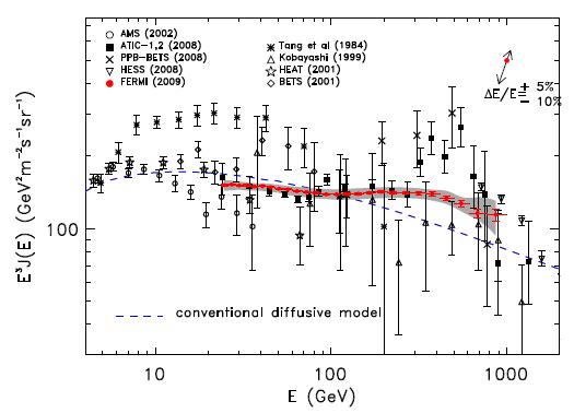
In the plot you get to see on the vertical axis the flux of electrons and positrons combined, measured as a function of the particle's energy (on the horizontal axis). The flux is multiplied by the cube of the energy, in order to flatten it out. Not merely an artificium for display purpose, since the cubic trend is more or less what the model predicts.
You have probably already realized that the one shown is a busy plot! It contains a mouthful of data from several different experiments. We should just forget about most of those families of points, and concentrate on the red points (the new Fermi data), and how they compare with the ATIC data (the crosses, showing a peak at a few hundred GeV). Please note that the theoretical "diffusive" model (one of many), which does not include dark matter annihilation, seems to predict a smaller flux than what Fermi observes in the high-energy range of its measurement; however, the difference is not too striking, if you look at the graph with a critical eye. These families of points are all over the place! For most of the past measurements of the flux, we used to be talking about order-of-magnitude estimates.
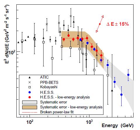
Now let us give a look at the HESS result. Here there are two families of points from the Cherenkov telescope: one is optimized for lower energy (in red), the other is more standard (in blue). HESS finds a sort of knee in the behavior of the flux, but its data does not disagree with the model:
To make a few points of the mass of information displayed above, let us start with the obvious. First of all, and maybe most important: the two new results agree, within uncertainties, among each other. They span slightly different energy ranges, as mentioned above, but they overlap significantly in the region they cover together. A colleague overlapped the two graphs with photoshop, and the result appears clearly -sorry, I do not have that combined plot available to show.
Second, the results also undershoot significanlty the energy flux measured by the ATIC collaboration, which seemed to show a suggestive bump in the spectrum. The ATIC bump, together with a similar measurement made by the PAMELA collaboration (this latter result does not get compared to Fermi and HESS results in the two papers, because it measures a ratio between positrons and electrons rather than a total flux of these particles) could be taken to indicate the annihilation of dark matter particles in the galactic halo, as I had a chance to discuss in a recent post. Since the new data are way more precise than those from ATIC, one has to reckon with the fact that the bump is gone.
In truth, Fermi does see some suggestive smooth bump in its data distribution; but the paper clearly explains that a straight-line fit to all their data points has a pretty large probability - so the no-bump is as good an explanation as any.
It is quite likely that the following weeks will see dozens of new papers appearing on the Arxiv: attempts to fit together all measurements, speculations on the shape of the spectrum, theories involving dark matter which discreetly sneaks in, and thus causing no smoking-gun signal in the energy distribution, exotic models whereby dark matter annihilates into electron-positron pairs only during months containing the letter R, etcetera. It will be nice to sit and watch this flurry of activity. To me, the Fermi and HESS results sound simply as the latest killing of a possible hint for new physics. Ah, Standard Model! We love you and we hate you... As Gaio Valerio Catullo superbly put it 2060 years ago:
Odi et amo. Quare id faciam, fortasse requiris.
Nescio, sed fieri sentio et excrucior.


Comments