Deriving the Maxwell Source Equations Using Quaternions (2/5)

The Maxwell source equations will be derived using quaternions - an approach James Clerk Maxwell himself tried and yet failed to do. As far as I am aware, this technique is not in the literature, up to an isomorphism (meaning actually it is there but under a different name, math in disguise). By using quaternions, the approach can be extended to generate field equations for particles with the weak and strong force symmetries, SU(2) and SU(3). The extension is a technical speculation, which I define as precise math whose applicability to Nature I have not a clue :-)

Warning: doing a classic field theory calculation in detail requires far more math than is customary on this site. The blog is my longest so far...
Click or Skip this reading of the blog
Start with the biggest possible picture - define what the Maxwell equations accomplish. The Maxwell equations detail all the spacetime changes in all spacetime changes in a spacetime potential created by massive particles in a spacetime current density mediated by particles that contain no notion of their own history, photons living in now. The fab four of equations have stunning staying power, riding from 1860 through special relativity, general relativity, and quantum mechanics unaltered. Those who have played in the ensemble grunge band "The Standard Models" know that they perform covers of Maxwell using louder groups in their Marshall stack of PR amps. Out here on the ultra-conservative fringe, I have zero tolerance for the new age noise that uses strings. Time for Dorothy to go home to Kansas field theory. Know Maxwell, know physics.

The next four blogs use the same three part harmony of steps. The first is to define the Lagrange density. This step needs contemplation - why should this particular small collection of symbols dominate the actors on Nature's stage? Given her creativity, completeness is a requirement. The second step is to run the one Lagrange density through the four Euler-Lagrange equations to generate four field equations. This is a graceful math machine whose details are rarely revealed in public due to the investment required to draw all the gears and levers behind the curtain. There will be a visual component to the exercise to limit the level of detail needed to see the Euler-Lagrange equation in action. The third step is to pick a gauge to reorganize variables on the bookshelf, making the results so neat and tidy they can be committed to memory. Lagrange density, Euler-Lagrange, choose a gauge: rinse and repeat.

Quaternions will be used to define the Lagrange density for the Maxwell source equations. A quaternion is a rank 1 tensor in four dimensions that comes pre-equipped with multiplication and division. Here are the rules for multiplication, since quaternions have been blacklisted from schools by the high priests of math textbooks:
$(\rm{first}, \rm{Last}) \times (\rm{first}, \rm{Last}) = (\rm{firsts} - \rm{lasts}, \rm{Outie} + \rm{Innie} + \rm{Cross})$
Note: the capitalized words are 3-vectors.

Construct a complete set of first order changes of a spacetime potential using quaternion multiplication:
$\begin{align*}(\frac{\partial}{\partial t},\vec{\nabla}) \times (\phi, \vec{A}) &= (\frac{\partial \phi}{\partial t} - \nabla \cdot A, \frac{\partial \vec{A}}{\partial t} + \vec{\nabla} \phi + \vec{\nabla} \times \vec{A}) \\ &= (gauge, -\vec{E} + \vec{B}) \end{align*}$
The electric field E and magnetic field B just show up. Luck? I'll take a pair of aces as my down cards. This is the simplest thing one can do with a quaternion derivative and potential, which gives me the most important fields in physics. Nice.

Some may complain about the gauge term. There is a time and a place for gauges, specifically the last blog in this series. This is not the time nor the place for a gauge, so subtract the terms into empty time oblivion:
$\nabla \times A - (\nabla \times A)^* = (0, -\vec{E} + \vec{B})$
By erasing the gauge completely, photons are allowed to fly at the speed of light c. They have no history to tell. This is a physics fact I accept, but have yet to develop a pithy pitch for a broader audience.

Those barely in the know about quaternions complain that quaternions don't commute. Things that spin have that property too. Everything I have ever touched spins in several ways. That bug sounds like a feature to me.

Time to counter-attack. Calculate the fields with the order reversed, seeing the effect of not commuting:
$A \times \nabla - (A \times \nabla)^* = (0, -\vec{E} - \vec{B})$
Whiners will weasel that we don't know which one to use. The definition of the Maxwell equations discussed earlier makes the answer clear: to be complete, both orders must be used. Form the product of these two:
$\frac{1}{4}(\nabla \times A - (\nabla \times A)^*) \times (A \times \nabla - (A \times \nabla)^*) = (B^2 - E^2, 2 \vec{E} \times \vec{B})$
While this might look complicated, the zeros in front make this easy: the first term is the negative of the product of the two, while the vector part is all cross product. The Lagrange density for the Maxwell source equation is the first term, the difference of squares. Poynting's vector which describes the energy density of the EM field shows up for free as the vector term. Like everyone but Poynting, I will ignore it. The difference of squares term is invariant under a rotation. Rotate, and B still points in the direction of B, while E points in the direction of E. I am still struggling to find why boosts leave difference unchanged. Everyone says it is, so I am flopping around looking for a personalized explanation of this technical detail.

Step 1 Summary and Foreshadowing

There are two ways to take the quaternion spacetime derivative of a spacetime potential. Eliminate the gauge term either way. Take the product of the two. The Lorentz invariant scalar is the Lagrange density for the Maxwell source equations. A different combination of the two ways to take the quaternion derivative of a potential will yield the Lagrange density for the Maxwell homogeneous equations in the next blog.

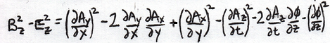
The Lagrange density B² - E² needs to be written out to its component parts. Bummer, there is a lot of detail there. This exercise has similarities to a Sudoku puzzle. There are some factors that can only show up exactly once per column. There are others that must appear exactly twice per row. The patterns can be used to check for errors.

Start simple, just as in Sudoku. Write out only B_x an E_x. Multiply those two together. Clone the pattern to figure out B_y and E_y. The values for z are then all fixed.

I cannot recall what goes into B_x, other than things that don't have an x. I have to write out the rule I learned by back high school:

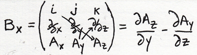
It is the Az term that is positive.

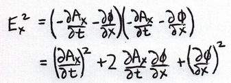
The electric field Ex I can recall: this has two terms, both negative, and they must both have an x factor:

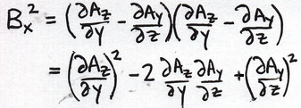
Square both of these:

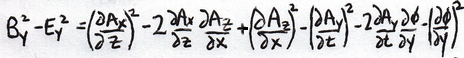
Subtract:

Each part of the 4-potential shows up twice. Each differential shows up twice. This is consistent with the completeness claimed for the Maxwell equations. I am writing this out by hand as an example of the only way to learn this process. Feel free to copy.

Do variations on this theme to do y and z:

Use the Sudoku rules on the columns to check my work (better if you copy to confirm).

There is a current coupling term that goes into the Lagrange density. It is easy by comparison:

In another blog I showed how the vector part implies a spin 1 particle is doing the work. Spin 1 particles mediate forces where like charges repel, perfect for EM.

One last detail: there needs to be a factor of a half in the difference of the squares of the two fields B and E.

All the parts are in place. Here is the Lagrange density written out in terms of its components:

There are twenty two terms in all.

Time to drop the 22 terms of the Lagrange density into the four Euler-Lagrange equations with 20 slots to fill. Ouch. Don't try to do everything at once quickly, that never works. Set up the ground rules first. There is lots of repetition in the Lagrange density.

Start with the two and only two bits of calculus that will be used over and over again in the next four blogs. Even if a reader has never taken a calculus class, these are often the first two rules one learns. They are dead simple. Start with a simple function like this:

$f=x * y$

In calculus, we want to know how the function f changes as x is varied. There is only one x, so the way the function f will change with respect to x is plain old y. To dress that up in fancy math clothes, we write:
$\frac{d f}{d x} = \frac{d ~(x * y)}{d x} = y$
The other example is ever so slightly more complicated. What happens if x = y, so we have:
$g = x * x = x^2$
A first guess might be that this function will just like the last one, and thus be equal to x. Close, but not quite. The rate of change needs a factor of 2 taken downstairs from the exponent:
$\frac{d g}{d x} = \frac{d x^2}{d x} = 2 x$
This is all the calculus needed to derive the four Maxwell equations and my two variations.

There are situations where a simple sounding question is hard, like what is inertia? There are others that look hard, but are simple. It is the second case that happens here time and time again. Instead of a simple looking factor of x, we put in a complicated looking thing. Even if complicated looking, it still turns out to be the x² -> 2x calculus party trick. Here is an example:
$\\ \rm{Let} ~x = \frac{d \phi}{d x} \\ \rm{Let} ~h = \frac{1}{2} \left( \frac{d \phi}{d x} \right)^2 \\ \frac{d h}{d \frac{d \phi}{d x}} = \frac{d \frac{1}{2} \left( \frac{d \phi}{d x} \right)^2}{d \frac{d \phi}{d x}} = \frac{d \phi}{d x}$
This is why I tossed in the factor of a half earlier, so it would collide with this factor of two from the calculus, leaving a one in its wake.

Scroll up and take another look at the Lagrange density. It is all the complicated looking xy and x² sorts of creatures. There is nothing there but those two types. The Euler-Lagrange equations plucks these out, and slaps on another derivative. The Euler-Lagrange equation turns into a second order derivative factory. There are no factors of two as they all get wiped out.

To derivative Gauss's law, one works with any term that has a phi in it. All other terms can be ignored. Nice.

Only the terms on the right are used. In the mind's eye, erase one term having a phi for all those highlighted, or more formally, apply the Euler-Lagrange equation:

This result can be written in a simpler way. When defining the Lagrange density, the time derivative of phi and divergence of A were deleted. We are thus free to pick a relationship between these two since it will not change this calculation in any way. Here is something called the Lorenz gauge (no t in the name):
$-\frac{\partial Ax}{\partial x} -\frac{\partial Ay}{\partial y} -\frac{\partial Az}{\partial z} = \frac{\partial \phi}{\partial t}$
Use this substitution to get the simpler looking Gauss's law in the Lorenz gauge:
$\\ \rho &= \frac{\partial^2 \phi}{\partial t^2} - \frac{\partial^2 \phi}{\partial x^2} -\frac{\partial^2 \phi}{\partial y^2} -\frac{\partial^2 \phi}{\partial z^2} \\ &= \square^2 \phi$
The box squared is known as the D'Alembertian operator.

Summarize the results:

That is the no-shortcuts-taken way to derive Gauss's law.

Repeat this process, this time focusing on any term with the Ax, ignoring all others:

These terms live in different places. Good, we want to have complete coverage of the Lagrange density. Erase terms in the mind's eye that have an Ax:

It is not trivial to pluck out the curl of a curl of A, a detail one would work through as a grad student. Instead, notice how it has the look of a curl of a curl, the shifts, the variations on x's, y's, and z's.

Summarize:

This is Ampere's law along x. Different boxes are used for the other two directions, but a similar story.

I will not show the details, but again one can choose to work in the Lorenz gauge, and again it rearranges things nicely:
$\vec{J} = \square^2 \vec{A}$

Compare the derivations of Gauss's and Ampere's laws:

What is fun about this visualization is that I can see things that might be missed with the pure algebra approach. For example, there is overlap between Gauss and Ampere involving the mixed terms of the electric field squared. Ampere's law hits the magnetic field mixed terms twice as well. All the pure squared terms are visited once.

How can we adapt this work to cover the symmetry of the weak force, the unitary quaternions? It is good that I know how to derive things. Look at the start of the derivation of the Euler-Lagrange equation from the previous blog:

1. Start with the Lagrange density. This must be one that depends on potentials and changes in potentials. A Lagrange density does not have to have this property.
$\mathcal{L}=f(A, \nabla A)$

Now we want to study a variation of this:

1. Start with the Lagrange density. This must be one that depends on normalized potentials and changes in normalized potentials. A Lagrange density does not have to have this property.
$\mathcal{L}=f(\frac{A}{|A|}, \nabla \frac{A}{|A|})$
How much is going to change in the seven step derivation? Nothing but how one writes the potential. Here is the unitary quaternion version of the Euler-Lagrange equation:
$\frac{\partial \mathcal{L}}{\partial \frac{A}{|A|}} = \nabla \left( \frac{\partial \mathcal{L}}{ \partial (\nabla \frac{A}{|A|})} \right)$
In all the wikipedia-level reading or discussions of the weak force, I have never seen a differential equation associated with the weak force. The discussions have always focused on symmetry, and the fun ways the weak force likes to break such symmetries. These are highly valuable insights. Yet take a look at the covariant derivative of the standard model:
$\mathcal{D}_{\mu}= \partial_{\mu} - i g_1 \frac{Y}{2} B_{\mu} - i g_2 \frac{\tau^i}{2} W^i_{\mu} - i g_3 \frac{\lambda^a}{2} G^a_{\mu}$
where
g = couping constant
Y, tau, lambda are the generators of U(1), SU(2), and SU(3) symmetry
B, W, G are the potentials for EM, the weak, and the strong force

The thing I wish to point out is the similarity of these three forces in the covariant derivative. All that appears to change is the symmetry group. It looks like there should be a Gauss's and Ampere's law that happen to have SU(2) and SU(3) symmetry. If so, they would start with a different Lagrange density, something like this:

Ouch! Kind of scary looking. There is a simple concept here: every darn term necessarily has unitary quaternion symmetry SU(2). Now I will repeat the derivation of field equations using the unitary quaternion version of the Euler-Lagrange equation.

No, this blog is way, way, way too long. You know what the result will look like, Gauss's and Ampere's laws.

To get to the strong force, do this swap in both the Euler-Lagrange equation, and the Lagrange density:
$A \rightarrow \frac{A^*}{|A|} \frac{B}{|B|}$
Everything will flow like the weak force.

The field equations can be written in the Lorenz gauge:
1. Maxwell source equations:
$J = \square^2 A$
2. The weak field source equations???
$\frac{J}{|J|} = \square^2 \frac{A}{|A|}$
3. The strong field source equations???
$\frac{J^*}{|J|} \times \frac{J'}{|J'|} = \square^2 \left(\frac{A^*}{|A|} \times \frac{B}{|B|} \right)$
The Maxwell source equations have been in the official canon of physics for over a hundred years. The field equations in 2 and 3 are technical speculations on my part. I have no idea how to test them.

To anyone lasting this long, congrats. Two of Maxwell's equations are down, and the method for getting the rest has been set up. Crank and go.

Doug

Snarky puzzle: This blog was too long. Make the author suffer. Let him figure out why B² - E² is invariant under a Lorentz boost.

Google+ hangout: 11:00-11:45pm Eastern time, Tuesday-Friday. http://gplus.to/sweetser

This could be an efficient way to exchange a few ideas. If you have a question or two, hangout.
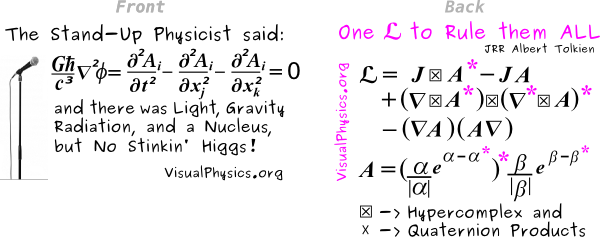
Bet against the Higgs being found, buy the t-shirt

Next Monday/Tuesday: Deriving the Maxwell Homogeneous Equations with Quaternions

Related articles

Comments

Know Science And Want To Write?

Donate or Buy SWAG