Diving into Euler-Lagrange: 1D (1 of 2)

Sophisticated physicists appreciate the dance of abstract symbols. I need to build something. The abstract is more real when made out of clay and pipe cleaners. In this blog on the 1D Euler Lagrange equations, beads (not clay) and pipe cleaners will be used to appreciate this important tool, followed by the same story told with symbols.

[note: I missed my usual self-imposed deadline because I was not able to get the icon bar to appear in Google Chrome on a Mac. The browser Opera worked, so long as I cut and plasted URLs for images and HTML code from codecogs.]

Calculus is the study of change. I will look into three variants. The first is differential calculus, the first one taught to students. The visualization is well known:

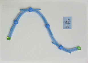
Notice the straight lines. This is a key to all forms of calculus - the linear approximation when changes are tiny enough.

Integral calculus involves summing. Its visualization should be familiar too:

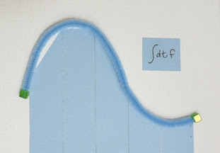
There are straight lines where the area bar meets the curve. The areas will become an excellent approximation when the changes become tiny enough.

The fundamental theorem of calculus can be viewed as the intersection of differential and integral calculus:

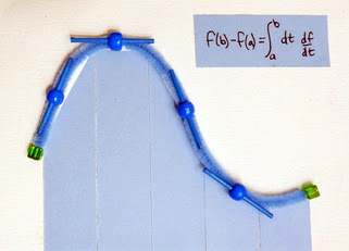
Take the integral of a derivative and the result is the function evaluated at the endpoints.

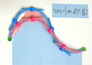
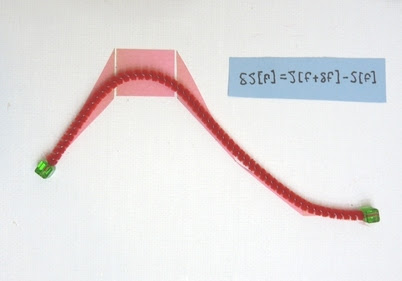
The calculus of variations is often not taught in a year long calculus class. One reason to avoid the subject is the focus shifts from one function to many possible functions and how they vary. This is quite the abstraction. The action to physicists, or functional [...] to math folks, can be visualized like so:

[Jargon correction sidebar]
I originally call the above a "functional integral" instead of a "functional". Turns out there is a BIG difference between the two. A functional is a function of functions. You may have seen something like this:
$f(a + b) = f(a) + f(b)$
This is true if f is an additive function. But the equation itself is called a functional equation. The calculus of variations is about minimizing functionals.Functional integration underlies the path integral approach to quantum mechanics. The math is much more difficult than is done in this blog. Often only perturbation theory can be used to get an approximate solution.
[End jargon correction sidebar]

Start with the function depicted by the line in blue. In both differential and integral calculus, that function, once set, stays the same. In [the action or functional], the function itself is allowed to change. One variation is the function shown in peach. It too has slopes, and those slopes are different from the ones in blue. The area under the curve can be larger or smaller depending on where one happens to be. The action S will be varying the function f which is why I wrote S[f]. What is "linear" is that one works with first order derivatives of the the function f, not higher order derivatives. I believe one can work with higher order derivatives, but that will be beyond the scope of this blog.

One comforting idea is that the tools of standard differential and integral calculus still work, with good old variables like position x substituted with alien functions like f. It can look like a global search and replace. For example:

$\frac{d x^2}{d x} = 2 x$

Likewise:

$\frac{d f^2}{d f} = 2 f$

The first derivative I ever learned still works even if I use a function f.

Another relevant tool is the method for looking for extremes, where the limit of a change is zero because a local maximum, minimum, or inflection point has been found. Here is a visualization of the process:

Compare three flavors of calculus: differential calculus, integral calculus, and the calculus of variations:

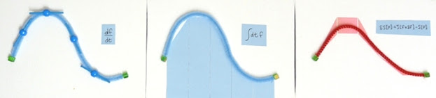
Differential calculus uses ratios. Integral calculus uses sums. The calculus of variations exploits both differentials and integrals when looking at [a small] difference [as the function is varied].

Enough with the pictures, on to the real mathematical physics.

Define the action S:

$S[f] = \int_a^b d t ~ \mathcal{L}\left[f, \frac{d f}{d t} \right]$

Original: Vary the function f by a factor of delta, looking at the limit of the difference like so:
Better I hope: The entire function f is allowed to vary by a small amount, δf. Over the entire range of the function f, the function changes. Look at the difference between the functional that is changing to first order in the derivative and the original functional:

$\begin{align*} \delta S[f] &= S[f + \delta f] - S[f] \\ \\ &= \int_a^b d t \left( \mathcal{L} \left[f + \delta f, \frac{d f}{d t} + \frac{d (\delta f)}{d t} \right] - \mathcal{L} \left[f, \frac{d f}{d t} \right] \right) \end{align*}$
[Two corrections were made to the original equation. First, I had put in a limit. What is really needed is the variation of the function must be small like the graphic suggests. This is so the variation depends on the first order derivatives of f, not higher order derivatives. Second, the delta needs to be snuggled against the function f because it is the function that is being varied. For a number of subsequent functionals, the limit process and location of the delta were altered.]

[note on notation: why not use f dot for the time derivative of f like everyone else? This is part of "owning" a derivation, writing it slightly different. This is forcing me to notice where the total and partial derivatives live throughout the process.]

What is the difference of these two in the integrand? Since the goal is to look at the [...] variation [for small changes in the function], one can take the Taylor series of the term on the left:

$\mathcal{L} \left[f + \delta f, \frac{d f}{d t} + \frac{d (\delta f)}{d t} \right] = \mathcal{L}\left[f, \frac{d f}{d t} \right] + \frac{\partial \mathcal{L}\left[f, \frac{d f}{d t} \right] }{\partial f} ~\delta f + \frac{\partial \mathcal{L}\left[f, \frac{d f}{d t} \right] }{\partial ~\frac{d f}{d t}}~ \frac{d (\delta f)}{d t} + O(2)$

The partial derivatives of the Lagrangian are used because the Lagrangian in this functional [...] depends both on f and changes in f (recall the picture). A derivative of the Lagrangian with respect to the function f must hold the time derivatives of f constant.

Plug the Taylor series expansion back into the variation, noticing the first term cancels, leaving:

$\delta S[f] = \int_a^b d t \left( \frac{\partial \mathcal{L}\left[f, \frac{d f}{d t} \right] }{\partial f}~ \delta f + \frac{\partial \mathcal{L}\left[f, \frac{d f}{d t} \right] }{\partial~ \frac{d f}{d t}} ~\frac{d (\delta f)}{d t} \right)$

I call this phase: apple (δf) meets orange ( d(δf)/dt). Pros can say integration by parts and boundary conditions and be done with it. Those who have to stay after school is out need to work through the details. I just don't use integration by parts on a regular or even irregular basis. I have an easier time with the product rule:

$\frac{d (a \cdot b)}{d t} = a \frac{d b}{d t} + b \frac{d a}{d t}$

or

$\frac{d (a \cdot b)}{d t} - a \frac{d b}{d t} = b \frac{d a}{d t}$

For that second term in the integrand, if a=f, and b is everything else - it is a bunch of stuff - then we can plug the two terms on the left for the one on the right.

$\delta S[f] = \int_a^b d t \left( \frac{\partial \mathcal{L}\left[f, \frac{d f}{d t} \right] }{\partial f} ~\delta f + \frac{d}{d t} \left( \frac{\partial \mathcal{L}\left[f, \frac{d f}{d t} \right] }{\partial~ \frac{d f}{d t}}~ \delta f \right) - \frac{d}{d t} \left( \frac{\partial \mathcal{L}\left[f, \frac{d f}{d t} \right] }{\partial ~\frac{d f}{d t}} \right) ~\delta f \right)$

This doesn't initially look like progress. There are now three terms instead of two. The middle term however is the fundamental theorem of calculus in action. It doesn't have to equal zero. However, physicists often pick boundary conditions such that this term is zero. If the boundary conditions are periodic, then the value will be the same at a and b, so the term contributes nothing.

[More detail on the "middle term" of the variation of the functional…]

$\int_a^b d t \left( \frac{d}{d t} \left( \frac{\partial \mathcal{L}\left[f, \frac{d f}{d t} \right] }{\partial \frac{d f}{d t}} \delta f \right) \right) = \frac{\partial \mathcal{L}\left[f, \frac{d f}{d t} \right] }{\partial \frac{d f}{d t}} \delta f \left|_b - \frac{\partial \mathcal{L}\left[f, \frac{d f}{d t} \right] }{\partial \frac{d f}{d t}} \delta f \right|_a$

Say the endpoints are fixed (there is a wall there, that kind of thing). Then the function f cannot vary at the endpoint b, nor at a, so this will evaluate to zero. In the graphic, the endpoints were green cubes that were epoxied to the canvas.

The endpoint could vary, but if they varied together, then again the middle term would evaluate to zero. This is what is meant by "harmonic boundary conditions": what happens at endpoint a is what happens at endpoint b, so these two are the same and cancel each other.

A third option is to say one is going out to infinity, and there is no there there (the Lagrangian is zero that far away).

[end detail]

Proceed assuming the periodic boundary conditions or things go to zero at infinity and beyond (I watch a lot of "Toy Story" these days). Apples are now together with apples:

$\delta S[f] = \int_a^b d t \left( \frac{\partial \mathcal{L}\left[f, \frac{d f}{d t} \right] }{\partial f} - \frac{d}{d t} \left( \frac{\partial \mathcal{L}\left[f, \frac{d f}{d t} \right] }{\partial ~ \frac{d f}{d t}} \right) \right) \delta f$

The variation of the action can equal...just about anything. What is of most interest to Nature is apparently extremums. That happens when the variation equals zero. And that happens if those two terms inside are always just as big as each other:

$\frac{\partial \mathcal{L}\left[f, \frac{d f}{d t} \right] }{\partial f} = \frac{d}{d t} \left( \frac{\partial \mathcal{L}\left[f, \frac{d f}{d t} \right] }{\partial ~\frac{d f}{d t}} \right)$

Is this extremum a maximum, a minimum, or an inflection point? That all depends on exactly what the Lagrangian happens to be. I have never seen that calculation done, a second derivative of this mess to see if it is positive, negative, or zero. There is always more to try out.

The odds are good that I have tripped over a detail or two since I have demonstrated low fidelity at these tests of symbol manipulations. I will keep the pipe cleaner canvases on the book shelf. The eye can appreciate the logic of the calculus of variations quickly.

Doug

Snarky Puzzle:

A few blogs ago in the comments section, a little finite group theory happened, leading to the calculation that the quotient group of the quaternion group Q₈ modulo the multiplication group {1, -1} Z₂ was the Klein 4-group:

$Q_8 / Z_2 = V$

Don't feel bad if that doesn't mean much to you. Instead reread the comments so that it will make some sense - I know I tripped over any detail I could before stumbling to the answer. Now calculate:

$Q_8 / Z_4 = ~?$

What is Z₄? It is a finite group with - you guessed it - 4 elements. There are a bunch of ways to represent the group. One applies to the complex numbers: e^{(i n pi/2)} for n between 0 and 3. The result should be a non-Abelian because a quaternion divided by a particular complex number will be non-Abelian. Which group? Don't ask me, I have not done the calculation yet, but it may be interesting.

Next Monday/Tuesday: Diving into Euler Lagrange: 2D, 3D, 4D (2 of 2)

Related articles

Comments

Know Science And Want To Write?

Donate or Buy SWAG