


Dependence between variables, even within their contemporaneous and extreme movements, are not limited to linear relationships defined through the Pearson correlation, ρ. The ρ is the most common correlation calculation and looks at the parameterized covariance between two random variables, and confines the result to within -1 and 1.
We discuss in our blog note here the method to consider ρ for more than two variables. On the other hand, the Spearman correlation, r, removes the marginal distribution of the parameterized data, by calculating ρ on ranked data values. Also along additional dimensions, it should be noted that there are other dependencies that can also take place, by incorporating conditional lagged values into the variable’s relationships.
Specific examples are in a range of sciences, and include patterns between human temperature and heart rate here, multidimensional physiological disorders here, or the Beveridge curve linking unemployment and job vacancies here.
The purpose of this note is to show how non-linear dependencies can develop between the extreme movements in contemporaneous variables. We use copula mathematics to better understand the underlying relationship and show how this appears in a wide range of practical applications, for example in medicine and finance. It should make intuitive sense that data should exhibit a degree of negative sinusoidal pattern within them, and that this would be impossible to detect through linear calculations.
Note that technically here the symmetry of the variables allows one to invert the axes that they are seeing the relationship through. And what would remain would be the same mirror image between the variables, however the non-linear function mapped to it still must be described as a negative sinusoidal. Not a sinusoidal (its negative) pattern. Linear algebra students recognize this as having an "onto" mapping as independent variable --> dependent variable or surjective, if every dependent variable value is the image of at least one independent variable value.
Note that technically here the symmetry of the variables allows one to invert the axes that they are seeing the relationship through. And what would remain would be the same mirror image between the variables, however the non-linear function mapped to it still must be described as a negative sinusoidal. Not a sinusoidal (its negative) pattern. Linear algebra students recognize this as having an "onto" mapping as independent variable --> dependent variable or surjective, if every dependent variable value is the image of at least one independent variable value.
Through the central core of one’s data, the (negative) sinusoidal shape is fairly linear, though the outer parts would then abruptly curve back towards a more accentuated regression line. These outer parts generally have higher tail dependency; meaning not that their correlations must increase in those boundary locations, but rather that there can be some more exotic relationship that is strengthened there. This avant-garde belief that our relationships constantly depend on our relative situation is captured in one of 20th century Frank Herbert’s science fiction novels, Children of Dune, “Some actions have an end but no beginning; some begin but do not end. It all depends upon where the observer is standing.”
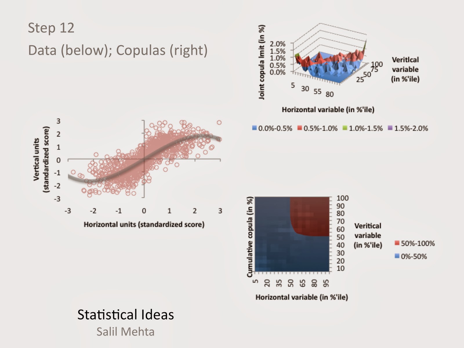
We’ve created the framework illustrated below to describe how we’ll effectively explore these overall and tail dependencies.
Shape high | Shape high-medium | Shape medium | Shape medium-low | Shape low | |
ρ = 1 | Step 1 | ||||
ρ = 0.75 | Step 12 | Step 2 | |||
ρ = 0.5 | Step 11 | Step 3 | |||
ρ = 0.25 | Step 10 | Step 4 | |||
ρ = 0 | Step 9 | Step 8 | Step 7 | Step 6 | Step 5 |
We start at step 12 and work our way to step 1, and the reverse the cycle back to step 12. We argue later that the while most research analysts are using modeling techniques within the “Shape low” area, the negative sinusoidal pattern is most apt in some cases and reside within the “Shape high” area. Specifically, close to the Step 12 intersection.
Before we show the video demonstration, we explain other components to examining the tail concordance pattern. Here we use a copula style of dependency formulas, which can work across many multivariate applications, even as we use the variation below for two variables:
F(x,y) = C(F(x) , F(y))
The Archimedean class of copulas can also work for two random variable families, including the Gumbel, and Clayton versions for exclusively upper or lower dependencies, respectively. The Archimedean copulas are likely named after the 3rdcentury BC Greek mathematician Archimedes, who alongside this class of copulas can be considered predecessors to more advanced knowledge in the mathematics field. Also for definitional purposes, upper dependency implies that higher values for random variables (death rate variables, or market change variables) tend to depend on one another. The lower dependency is when the opposite is true, so implying lower values for random variables tend to depend on one another. The copula function was the average. Both the simple, and the more conservative harmonic, averages were examined. We can use the averaging approach since the video below will illustrate the joint copula function, at the intersection of both variables’ marginal copula function.
Also note that while theoretically we may see an exclusively upper or lower dependency for the death data, or the financial market data, this was not borne out in the empirical data of the prior decade. For clarity one can reference still sample images for steps 12 and 4, respectively, right below the multimedia.
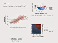
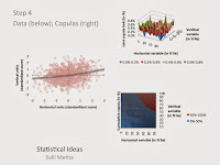

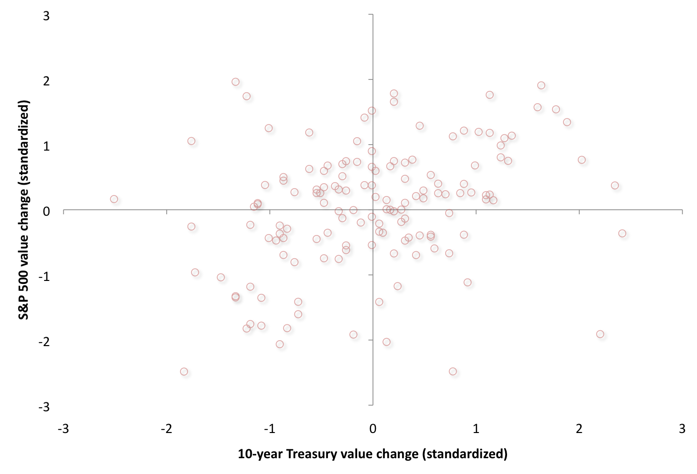
On the left we see the data construct for the two random variables. Over 1000 simulations were developed for each of the 12 steps. All the simulated and empirical data will be processed through a standardization procedure such that the distribution of all of the independent and dependent variables will be centered about zero and have a standard deviation of about 1. Additionally the display charts will be censored outside of the range of -3 to 3, thus incorporating more than 99.5% of the underlying distribution. On the right we show to copula charts, that we have earlier described. Thec(F(x),F(y)) joint copula on the top right, and the C(F(x),F(y)) cumulative copula pattern on the bottom right. We’ll also see that when the ρ=0, along the bottom row of scenarios (e.g., step 5 through step 8), there is little statistical differentiation that can be accomplished with the concept we’ve described in other posts as a high “variance about the hypothetical mean”.
It is evident in the multimedia illustration that because of the combined upper and lower dependencies, our overall results will look similar to that of a Student-t copula, which is also acceptable for the datasets examined here. But we shouldn’t be confused then in our conclusions since it can not be a symmetric Student-t itself when there is clear asymmetric skewing of the data as described above as a negative sinusoidal pattern. A more advanced understanding of the tail dependency pattern is to recognize that here we picked variables that had a positive overall relationship. So they emulate something between the minimal copula and independence copula to define its structure.
Now let’s see how this model construct we have developed fits the patterns within real world applications. We explore two data sets, one medical death data, and the other concerning financial market returns data. Both have their risk patterns directed in concordance to major outside risk factors, mostly nutrition, and proxies for economic patience, respectively. And both types of data tend to have variables that move together simultaneously, over the prior decade, within the data frequency we have captured.
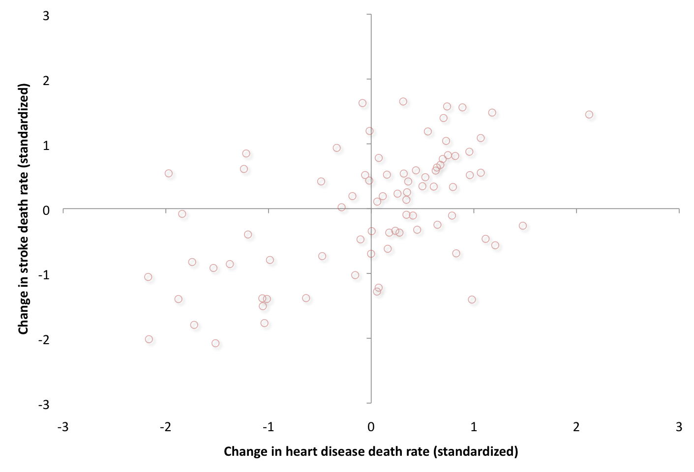
The first data set, from the CDC and NCHS, looks at the relationships between the change in death rates from heart disease (horizontal dimension) and the change in death rates from stroke (vertical dimension). The coefficient of variation,CV=dispersion/average, were equal for both variables. We look at nearly 80 aggregate U.S. data, between 2000 and 2010, from all of the U.S. federal health districts. We also highlight in the second of two illustrations below, the tectonical areas of the highest copula dependency function (in white).


And the second data set looks at the relationships between changes in the U.S. long-term Treasury yields (horizontal dimension) and changes in U.S. equity prices (vertical dimension). As can be expected, the CV was higher for the equity market changes versus the bond market changes. We look at nearly 150 aggregate US data, also between 2000 and 2010. Similar to the heath data presentation above, here we also show in the second of two illustrations below, the tectonical areas of the highest copula dependency function. We see through the symmetrical mapping and the recent year empirical data that we have a convex volatility function that is progressively generating a larger absolute S&P variance, given -a proximate in time- any greater relative bond yield variance.

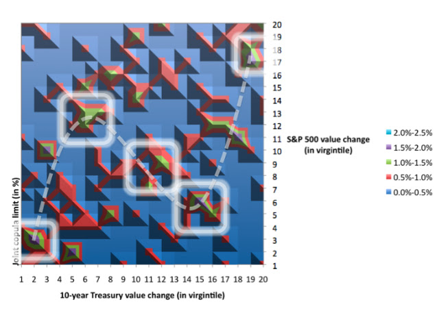
Both of these data sets show that the step 12 scenario mapped above (with the slight dampening, negative sinusoidal pattern) is the primary engine exhibited here. The dampening implies that there is enhanced amplitude in the lower tails and reduced amplitude in the upper tails. So in summary without the tail concordance patterns formulated here, research analysts would likely be confined in their modeling of risk patterns from empirical data, using only standard and theoretical, multinormal linear frameworks, such as steps 2 or 3. This linear-only approach is flawed and amounts to missing the exotic and important tail dependencies, which exist under the hood.


Comments