

This is a quite common setup in many searches in Physics and Astrophysics: you have some detection apparatus that records the number of phenomena of a specified kind, and you let it run for some time, whereafter you declare that you have observed N of them. If the occurrence of each phenomenon has equal probability and they do not influence one another, that number N is understood to be sampled from a Poisson distribution of mean B.
Now, in most cases you assume you have a model, or some data-driven algorithm, capable of predicting B. This automatically allows you to evaluate the probability of your observation of N: that probability is simply given by the Poisson function P(N|B) = exp(-B) * B^N / N! , where N! is the factorial of N.
However, P(N|B) is not a very informative number by itself: for large B, there are a large number of similarly probable outcomes for N, each of very small individual probability. Much more interesting is to assess what is the cumulative probability that the observed counts, given B, be at least as large as the value that was actually observed. This is what a classical statistician will use to appraise how odd it is to have seen an upward fluctuation of B up to N. It is called a tail probability, and it can be computed as
which is much better than summing up an infinite number of terms P(i>=N|B) for any integer i!
The P number above has more relevance as a test of the hypothesis that the process you have been recording counts from has indeed a rate B: if P is very small, N can be said to be significantly larger than B. In fact, one can directly use the above P as a p-value, and if need be convert it into a number of standard deviations. So, e.g., p=0.0017 corresponds to a 3-sigma significance, and p=0.000000297 corresponds to a 5-sigma significance, for what is called a one-sided test - when, i.e., we are interested in excesses of events.
The above is elementary and you can write in a minute a piece of code that computes P given B and N. However, B is never known with no uncertainty: either you have a model for it, which is by definition uncertain to some degree, or you derive B from an ancillary experiment. A typical setup of the former situation is a high-fidelity simulation of the process under study. The latter is instead exemplified by a detector watching a certain area of the sky (a signal region, where we are searching for a source of photons, e.g.); if we point the detector elsewhere, where we may assume there is no source of photons, we get an estimate of the counts from backgrounds alone in the signal region by counting photons for the same amount of time.
Allowing for B to be variable -say with uncertainty sigma_B- complicates the problem quite considerably. A classical statistics way of solving it is to sample a realization B' from a Gaussian distribution of mean B and width sigma_B, and proceed to compute in each case P(>=N|B') as above; then one may obtain an estimate of P(>=N) by dividing by the total trials. However, already here are hidden a couple of small devils. The first one: one must average all P values, not be happy with a median! And secondly, what does one do if sigma_B is not very small compared to B? A Gaussian extends its tails to minus infinity, endangering our numerical calculations if we end up with a negative Poisson mean...
It transpires that we should abandon the idea that we may know B to within a certain additive shift (along with its resulting Gaussian model of G(B,sigma_B)) and rather pick a more motivated distribution of possible values of B'. A log-normal distribution (which is the result of the product of many small multiplicative shifts, and is thus much more appropriate to model uncertainties in a positive-defined number) certainly be a better motivated choice, but already in admitting this one is faced with the fact that the result contains arbitrariness - in the choice of the density function of the possible B values.
All that said, our piece of code modeling a log-normal uncertainty will probably be 15 lines long instead of 5, and we can still effectively solve numerically our little problem even if we are given a uncertainty sigma_B on the expected counts B. This is what I have given as an exercise to my students over the past few years. Funnily enough, recently I found myself struggling with the same problem! The reason is that I needed, for a detector optimization task I am working on, a differentiable function that describing the number of events corresponding to a 3-sigma excess, given background B and uncertainty sigma_B. The requirement of differentiability prevents (although I should rather say discourages) you from obtaining the function by random sampling.
The differentiability requirement serves the purpose of allowing me to define a utility function - in this case U=1/N(3-sigma), i.e. a quantity that is larger if the number I need to observe to have a 3-sigma excess is smaller. This situations occurs if one e.g. wants to be sensitive to smaller signals. By having U differentiable, I can compute its derivative with respect to the geometry of my apparatus, and optimize it.
In the literature you can find a number of exact as well as approximated formulas for the significance of a counting excess, under various guises and situations. There is the Punzi significance, the Approximate Median Significance, the On-Off problem significance of Li and Ma, and a plethora of numerical approximations that have different merits and are simpler or harder to compute. While the On-Off solution of Li and Ma constitutes a valid starting point, as it is the closest to the actual setup of my problem (I am indeed counting events from a source of gamma rays in the sky, the same problem discussed by them), it only considers Poisson uncertainties in the value of B (which is extracted from an off-source measurement). In reality, a systematic uncertainty on B which may have different sampling properties is not so uncommon.
As I lacked the time to perform a complete analytical solution of the problem -and was unsure of whether I would end up with a differentiable result in the end anyway- I took another route. I computed the significance with the code I give in my example solution at the PhD course for a vast number of combinations of B and sigma_B, which exhausted the cases I was interested in, and proceeded to fit the resulting N(3-sigma) values as a function of sigma_B for each value of B with a simple analytical form (a power law); then I extracted the parameters of the power law and proceeded to fit those, as a function of B. In the end I got a quite simple analytical form for the number I sought.
Below are a few sample fits to the N(3 sigma) values as a function of sigma_B, for different values of B: top row, left to right, we have 5, 10, 15, 20, 25 expected counts, and the x axis spans relative uncertainties ranging from 0 to 30%. On the bottom row we get the distributions for B ranging from 30 to 50, in 5-event steps.
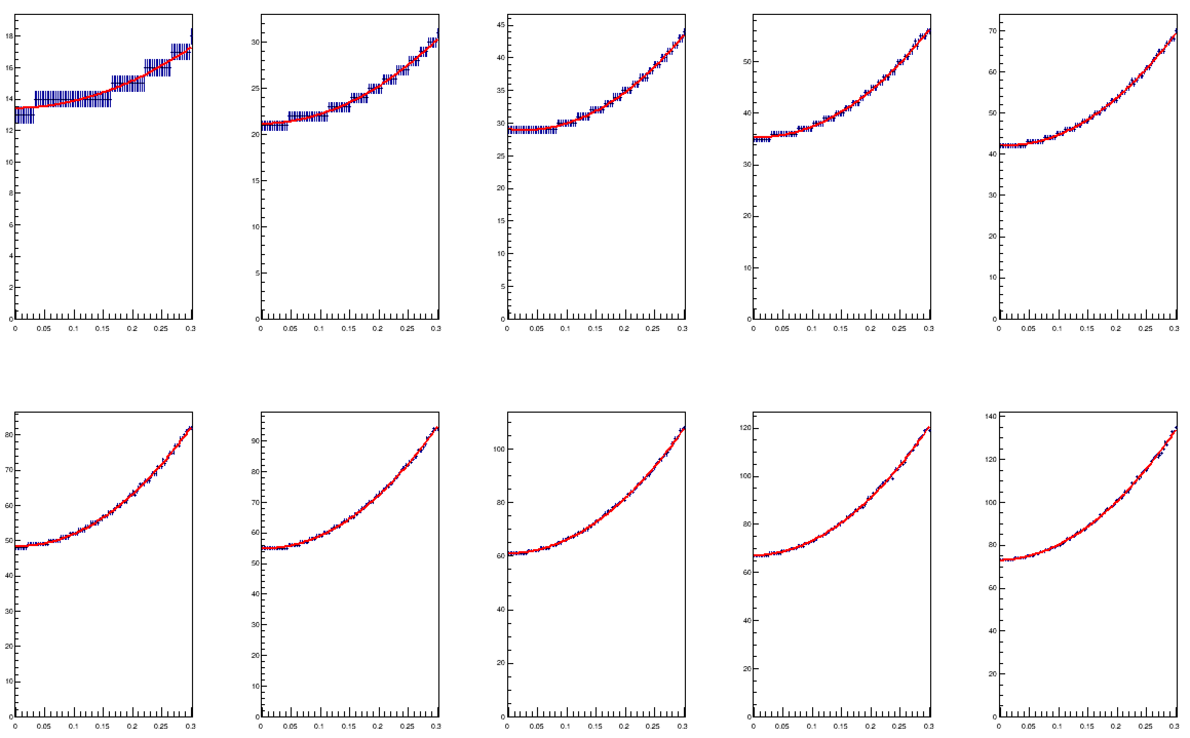
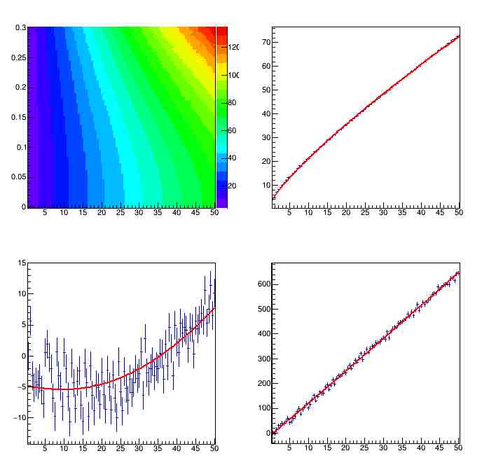
As you see, the fits are a reasonable model of the 3-sigma threshold, for the considered space of parameters [B,sigma_B/B] = [[0,50],[0,0.3]. Now to get a model of N(3-sigma) valid for any B and sigma_B/B combination we need to interpolate the fit parameters of the above power law functions. This is shown in the graph below.
The three parameters show a bit of bumpiness - especially the second - but the quadratic fits are sufficient for my task. The top right panel shows a temperature map of the values of N(3-sigma) as a function of the two parameters in the exact model, the three parameters are instead shown as a function of B in the top right, bottom left, and bottom right panels.
Finally, we can check how different the model is from a simple-minded approximation that considers a Gaussian approximation of the Poisson distribution, and just evaluates N(3-sigma) as B + 3*sigma_B. I care to show it below as it is instructive to study the graph.
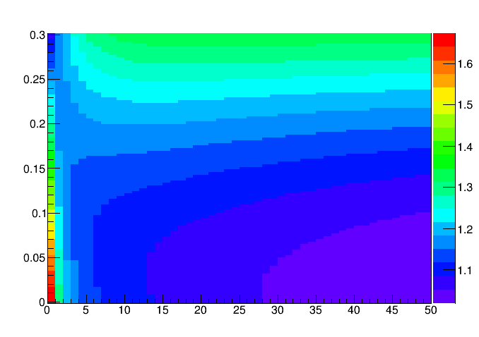
Here the x axis shows the studied values of B, and the y axis shows the relative uncertainty sigma_B. The colour on the graph shows the ratio of the approximated model I came up with to the Gaussian approximation. As you can see, when B is large and sigma_B is not large, there is a good agreement of the two values. However, bump up sigma_B to a significant fraction of B, and the Gaussian approximation starts to under-predict N(3-sigma). For small values of B the effect is instead more dramatic when sigma_B is small, as the peculiarities of the Poisson distribution create a starker disagreement when there is no uncertainty on B.
Although the above model is rather imprecise in some specific regions of phase space, it is perfectly adequate for a Utility calculation in an optimization problem, where what matters is the derivative of the utility rather than its exact value. With this in the bag, I can happily move further with my project.


Comments