

The interest of measuring these decay probabilities is essentially due to the fact that a discrepancy of the measured rates with their respective theoretical predictions would betray the existence of something we have not yet included in our theoretical model: "new physics". This might be, e.g., the existence of new, as-of-yet undiscovered or even unhypothesized subnuclear particles, or new fundamental interactions. Particle physicists do this as a routine: when the accepted model allows a precise prediction of something experimentally measurable, they go out and measure it, as this provides stringent tests of the theory.
Indeed, if am allowed a digression, we have been investing a very considerable effort into the improvement of the measurement of a property of muons called "anomalous magnetic moment". That is another number that can be estimated with very high precision with SM calculations, and a comparison with the result obtained a decade ago by a dedicated experiment at Brookhaven Laboratories showed a mismatch which arises by chance less than once in a thousand trials. Now a new, improved measurement is being carried out at Fermilab. If the discrepancy will be confirmed, we will have a proof that there is something new to discover in the phenomenology of elementary particles, and will then start figuring out ways to go hunting for it.
The discrepancy between calculated and measured value of the anomalous magnetic moment of the muon is _the_ one place where the Standard Model seems to be breaking down. No similar situation exists yet in the phenomenology of the Higgs boson, but that's not a reason for not looking further: in fact, with the large amounts of collisions recorded by ATLAS and CMS in the past three years, we have a chance to look much more precisely into the matter.
ATLAS just did that with precise bounds on the H-->ee and H-->eμ decay rates. They did it by selecting events containing a signature of the two final state leptons, compute the mass that a hypothetical particle would have if it had decayed into the observed pair, and examine the resulting mass spectra. A bump at the Higgs mass value (125 GeV) would allow a measurement of the rate; its absence allows for a statistical procedure which extracts a so-called "upper limit" - basically a statement that the rate must be lower than X for the spectrum to look like it does.
Below you can see the mass spectra resulting from looking for electron-positron pairs (left) and electron-muon pairs (right). As you can see, both spectra look smooth, with no indication of a peak at 125 GeV. The lower panels in both graphs show the residuals, bin by bin, of the data subtracted by the background model produced by a likelihood fit. The red curve in the upper panels instead show what contribution one would have expected from Higgs boson decays with a rate of 2% (left) or 0.05% (right).
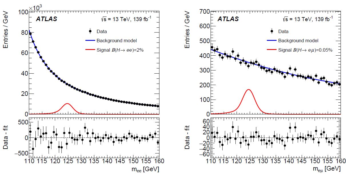
The contribution of Higgs boson decays would be much more visible in the case of electron-muon pairs because there the background is much smaller (you can see that also by checking the vertical scale of the two plots). Indeed, while in the case of electron-positron pairs the background is large and it is essentially due to Z decays, when the Z boson carried a rest energy exceeding its nominal mass of 91.2 GeV, in the case of electron-muon pairs the background is primarily due to heavy flavour decays (mostly top quark pairs, and it is less frequent after simple selection cuts are placed on the data.
Bonus track: why categorizing your data in different S/N subsets ?
One technical detail about the graph is that it is only a summary - in reality, ATLAS fitted separately seven (for ee) and eight (for eμ) different categories of event sets, depending on the additional features the events displayed. This kind of "divide et impera" approach improves the sensitivity of the search whenever the subsets have different expected signal to background ratios. This is a subtle statistical analysis point, but it can be appreciated with ease by considering a simplified example. Since I have nothing better to write about at this point, let me turn didactical and explain it below.
Consider a situation where you have expected number of signal events S and background events B. The presence of the signal produces an excess over background-only predictions, whose statistical significance can be approximated in the large sample limit as the ratio Z=S/sqrt(B).
[Warning: don't do this at home - the approximation really should only be used for large S and B!! Much better and still simple approximations exist, ask me about it if you are interested].
Now let us consider two cases below.
1) Imagine you can divide the S+B dataset into two parts without affecting the S/B ratio in each. You then expect that you will have S/2 and B/2 events in each subset. The significance in each will now be 0.5*S/sqrt(0.5*B), which turns out to be Z1, Z2=Z/sqrt(2). If you combine those two significances in quadrature, (again assuming large-sample statistics) you get a combined significance of Z12 = sqrt(Z1^2+Z2^2) = Z: nothing has changed. Doh!
2) Imagine instead you can divide the S+B dataset into two parts, such that the S/B ratio is k times higher in the first (with k>1). In general you can also choose how to distribute S in the two subsets, so you will e.g. write S2=f*S and S1=(1-f)*S, with f a number between 0 and 1.That means that you will have the following equations:
S1 + S2 = S
B1 + B2 = B
S1 / B1 = k * S2 / B2
S2 = f * S
S1 = (1-f) * S
The parameters k and f describe all possible partitions. Now, with some simple algebra, we can derive that
B1 = B * (1-f) / [1 + f * (k-1)]
B2 = B * k * f / [1 + f * (k-1)]
We can then derive that the significances Z1 and Z2 in the two subsets are
Z1 = S1/sqrt(B1) = sqrt [(1 + f * (k-1)) * (1-f)]
Z2 = S2/sqrt(B2) = sqrt [(1 + f * (k-1)) * f / k]
By combining them as before, we get the equivalent significance as
Z12 = sqrt (Z1^2+Z2^2) = Z * sqrt [ (1 + f * (k-1)) * ( 1 - f + f/k)]
That still looks complicated, but it really isn't. Let us just pick k=2 (remember, k>1 is how much larger is the S/B ratio in the first subset than in the second), and this simplifies to
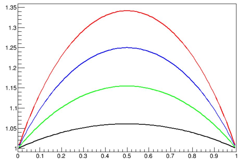
Z12 (k=2) = Z * sqrt [1-f/2 -f^2/2]
The function is shown in black, for any f in [0,1], in the graph below, where the vertical axis is in units of Z, the original significance of the full sample. As you can see, the function is always larger than 1, meaning that the combined significance of the two unequal-S/B subsets is always larger than Z=S/sqrt(B). In green the function is shown if k=3, and in blue and red the cases of k=4 and 5 are also shown. Notice how the larger the difference in S/B ratio of the subsets you extract, the higher will your significance be, for any f. You can also clearly see that the best situation for you is if you manage to keep the fraction of signal in the two subsets equal (i.e., f=0.5). So keep this in mind the next time you design a categorization of your data: strive for the highest k you can get when f=0.5!
---
Tommaso Dorigo is an experimental particle physicist who works for the INFN at the University of Padova, and collaborates with the CMS experiment at the CERN LHC. He coordinates the European network AMVA4NewPhysics as well as research in accelerator-based physics for INFN-Padova, and is an editor of the journals Reviews in Physics and Physics Open. In 2016 Dorigo published the book “Anomaly! Collider physics and the quest for new phenomena at Fermilab”. You can get a copy of the book on Amazon.


Comments