
This is part #3 of a brief explanation of the NASA/GSFC MODIS Rapid Response System - Rapidfire - together with a Howto for citizen scientists. The first parts were -
MODIS Rapidfire For Citizen Scientists - #1
MODIS Rapidfire For Citizen Scientists - #2
In this part, I'll show you some more tips on using the Arctic mosaic and images from the various bands available.
Pinpointing the North Pole
Why is this important? If you can locate the pole in any downloaded near-real-time images, you can rotate any image to place North at the top, which is the mapping convention in most countries. It can also help alignment if you want to stitch together your own mosaics.
The pole is in the middle of the mosaic, obviously. In an image manipulation program - imp - you usually get a cursor tracker. If you know the image size, you can find the exact centre. When viewing the mosaic online, there's an easier way. Just right click somewhere near the pole. Get rid of the menu by clicking on the frame of your browser. You should now see something like this. Without the red circle showing the pole, of course.
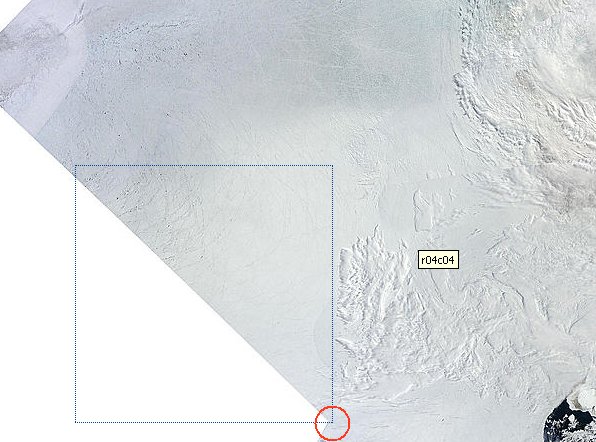
Location of pole in mosaic.
The pole is at the point where four images come together. It's useful to know that, just in case your imp doesn't have a cursor tracker. You can just eyeball a speck of cloud or other feature and get a fairly good idea where the pole is in your downloaded images.
The individual images first shown in the Aqua and Terra Near-real-time production images section have an overlay which helps you to guess where the pole is.
Image sizes
To recap from part 2, you can view the mosaic in 1, 2 and 4km resolutions as a 6 x 6 grid or as a single image. The single image is best for downloading. In the grid view, once you click on a row and column you get a view of that section only. The default size is 1km per pixel, but you can select any of 4, 2, 1, 0.5 or 0.25 km.
Once in a while you will want an image at 0.25km which straddles two mosaic sections. Rather than stitch two images together, I usually switch to Near-real-time production and browse for an image with the feature in the middle vertical third - the least distorted part.
Blinking images
Before the computer came into widespread use, astronomers both amateur and professional would use a blink comparator to compare images. The gadget could be as simple as a light box with a hinged mirror. The viewing of alternate images of a pair would make an object like a meteor or asteroid seem to jump in the image, for example.
Using the same principle you can compare any two images. Arctic watchers often choose two different dates and make an animation. That can be pretty spectacular.
North West Passage June 2009 compared with 2010
image credit: neven
If you take any two compatible Rapidfire images, you can usually get a useful effect.
An animation made from the same day's aqua and terra images will emphasize clouds. This can be very useful for spotting the difference between ice and cloud at a glance.
Arctic mosaic, aqua and terra animation June 19 2010
.
Once you know what is cloud, you can see at a glance the difference between the colder, more compact and less melted central ice mass and the bluish, heavily fragmented surrounding ice.
I shall zoom in on the details in part #4. For now, I continue with some more hints on blinkmaps and animations.
Mixing bands
If you save an image created from different bands, you can make a blinkmap to emphasize any feature. For example, this next blinkmap emphasizes the differences between ice, land, open water and clouds. The band of dots to the right draws attention to areas of fragmented ice.
True color image and bands 3-6-7
The next image emphasizes what I call ice quality, or lack of quality, as well as clouds and surface meltwater.
True color image and bands 7-2-1
Now that your attention has been drawn to various areas of the ice, you may wish to check out the original image at various resolutions:
http://rapidfire.sci.gsfc.nasa.gov/realtime/single.php?T101720345
Using image processing to enhance features
In any reasonably good image manipulation program you will find tools for image processing. It is worth experimenting with them. The method is to make a copy, B, of image A. Image B is processed and then animated with A. Here is just one example. Using a median cut noise filter removes 'speckle' - the parts of the image which show mainly as small dots. Here is an example animation using the median cut.
Humboldt Glacier and Kane Basin.
The glacier front is the line between the blue and the white ice. Behind the front, the blinking draws the attention to the meltwater pools. At the bottom right, a lead is emphasized. That huge ice island is not attached to the land and will soon be on the move.
In the main water area, the blink emphasizes the fainter specks which might otherwise escape attention. Look especially at the bottom left. To software, that area might well be seen as 90% concentration. To the human eye, it is ice being melted and flushed out of the Nares Strait. In estimating ice quality, much of the ice in this image can be entirely discounted. It is a hazard to navigation, but it is extremely unlikely that this highly mobile ice will survive to take part in the next winter freeze. Note also that thousands of the small dots will be icebergs, not sea ice.
In part #4 I'll show some closeups of ice types and features to help you analyze the images. Meanwhile, here is an image which shows how little of the Arctic sea ice can justifiably be considered as a 100% concentration. If you go to the mosaic and look at various parts in high resolution, you will see fragmented ice, meltwater, leads etc. in all areas outside the large circle. The smaller circle is, of course, the pole.
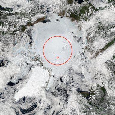
Area of maximum ice quality - June 19 2010
Source image:
http://rapidfire.sci.gsfc.nasa.gov/subsets/?mosaic=Arctic.2010170.aqua.4km
To be continued ...
-----------------------------------------------------------------------------
Credit:
All images courtesy the U.S. taxpayer and NASA/GSFC, MODIS Rapid Response
http://rapidfire.sci.gsfc.nasa.gov/.


Comments