

And even today, following three centuries of discussion and debate, the problem continuous to intrigue scientists and lay people alike. Yet, the paradox got fully resolved in the middle of the previous century. I was reminded of this paradox when it came up here at Science 2.0 in the comment section of a recent blog post on math paradoxes. When I checked the Wikipedia page dedicated to this paradox, I was shocked to see that this article mentions several approaches that have been claimed to resolve the paradox, but relegates the real resolution to this paradox to a short remark.
Time for a blogpost.

Imperial Academy of Sciences, St. Petersburg
St. Petersburg Lottery
The rules of the St. Petersburg lottery are straightforward: a fair coin is tossed repeatedly, until a tail appears, ending the game. The pot starts at $2 and is doubled each time a head appears. After the game ends, you win whatever is in the pot.
So if the first coin toss results in a tail, you get $2. A head followed by a tail pays you $4. Head-head-tail yields $8, etc. Now the question is: how much are you willing to pay to enter this lottery? Statistical reasoning tells us to compute an ensemble average: investigate all potential outcomes and calculate the sum of the gains for each outcome weighted with the probability for that outcome. This weighted sum is known as the expected gain.
For the St. Petersburg lottery where one wins $2 with probability 1/2, $4 with probability 1/4, $8 with probability 1/8, etc. the expected dollar gain is
(1/2) 2 + (1/4) 4 + (1/8) 8 + (1/16) 16 + ... = 1 + 1 + 1 + 1 + ... = infinite
The divergence of the expectation value means that no finite amount suffices as a fair entry fee for this game. Yet, if you play the game, you are sure to win no more than a finite amount. Also in actual practice, participants subjected to this game are not willing to pay more than a small entry fees (typically less than $20).
What is happening here? Why is the expectation value for the St.Petersburg lottery such a poor representation of human actions in this lottery?
Interestingly, the resolution to the St. Petersburg paradox becomes particularly transparent when applying statistical physics insights.
Steinhaus Sequence
Although I present the results in statistical physics language, the argument below follows the essence of Hugo Steinhaus' 1949 paper. It helps to investigate a simpler, deterministic game that shares its key characteristics with the St. Petersburg lottery.
Imagine an infinite sequence of powers of two. The numbers generated follow a deterministic rule, that is recursive in nature:
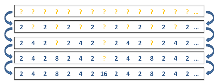
1) Start with an endless list of empty states and the number '1'
2) Double the number and, starting with the first empty state, fill every other empty state with the number
3) Repeat step 2) ad infinitum
Building a Steinhaus sequence
So we get a sequence that starts with the number '2', followed by a '4', then a '2', an '8', a '2', a '4', etc. If you would select at random one of he numbers generated, you would half of the time hit a '2', one quarter of the time a '4', and so on. Therefore, the expected value of numbers in the Steinhaus sequence is no different than that for the St. Petersburg lottery. More specifically, the Steinhaus expectation value diverges in exactly the same way as the St. Petersburg expectation value.
However, one may also ask what value we would obtain when averaging over subsequent numbers in the Steinhaus sequence. For the first two numbers, an average value of (2 + 4)/2 = 3 is observed. For the first four numbers we have (2 + 4 + 2 + 8)/4 = 4. Averaging over eight numbers we have (2 + 4 + 2 + 8 + 2 + 4 + 2 + 16)/8 = 5. We see a simple pattern developing. For 2n subsequent numbers we observe an average value of n + 2. This goes against the widespread intuition that the average gain per game should be independent of the number of games played. At least we expect this to be the case when the number of games played is large. Here, such is not the case.
Statistical physicists are familiar with this phenomenon. They refer to this peculiarity as 'non-ergodicity'. Ergodicity means that one can replace time averages with ensemble averages. Here, ergodicity does not hold as the time averages (the average values n+2 observed over 2n subsequent numbers) do not coincide with the ensemble average (the divergent expectation value). What is happening in any finite Steinhaus sequence, is that it visit large values contributing strongly to the average only logarithmically slowly, thereby causing a breakdown of the ergodic assumption.
Ergodicity
Now back to the St. Petersburg lottery. Based on the learnings from the Steinhaus sequence, it is easy to observe that also a sequence of gains from a repeated St. Petersburg lottery shows a pronounced breakdown of the ergodicity assumption. It is straightforward to generate a long sequence of St. Petersburg lottery pay-offs. This can be done with a coin, or more efficiently with any spreadsheet program. As suggested by the Steinhaus exercise, we plot the average gain of the first 2n numbers for progressively larger values of n. This is done in below figure for n up to 15 (2n = 32,384) for two independent runs.
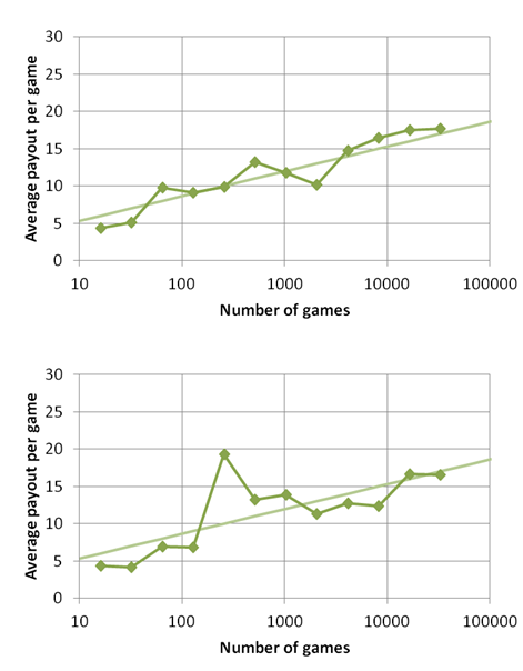
Although the average gains within each run fluctuate considerably, it is clear from the trends that the expected gains per game increases logarithmically with the number of games, just as we observed in the Steinhaus example. (To guide the eye, I have included in a fainter color the curve describing a pay-out per game of n+2 for 2n games.)
The conclusion is straightforward: only one type of averages are practically relevant in the St. Petersburg lottery. These are the the time averages. The St. Petersburg time averages are finite, but logarithmically dependent on the number of games played. As these time averages don't converge to a finite value in the long time limit, the ergodic hypothesis breaks down for St. Petersburg lottery results. Therefore, the ensemble average, aka the expectation value for the game, can be cast aside as a meaningless divergent quantity.
Math is simple if you're a physicist...


Comments