[Title correction: My goal was to create images of 2D, 3D, and 4D functionals. I think I missed that target. Instead I have 1D parameterized curves that all move in up to 3D in space + time. I have a clear idea how to write new code that could move independently with two, three, or four parameters. That code is not written now, so I will change the title to more accurately reflect the content.]

Nothing like writing a title where I am not sure if I can pull it off. It reminds me of skiing slowly off a 6 foot cliff in Colorado. By the time I landed, I was going fast. Nothing like the constant acceleration of gravity.

One, Two, Three D

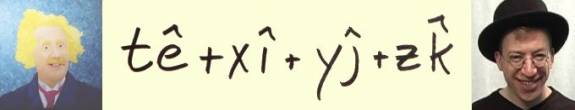
A one dimensional functional was easy enough to illustrate:


The endpoints are fixed with epoxy. The function itself is varied, but not by much (technically, only the first order derivatives come into play). The derivatives are the best straight line approximation at any given point of the function. The integral is the best linear approximation of the area under the curve.

For a two dimensional functional, there should be another pair of endpoints, for a total of four. There should still be the derivatives as slopes and the integral as an area.

[Corrections: If the function is the pipe cleaner, then this is a 1D parameterized closed loop in a 2D space. The endpoints are in the same place, should only appear as one cube. If the function were considered to be the area in pink, then the pipe cleaner becomes the boundary. The derivatives would not be lines, but squares. The integral would be some kind of volume.]

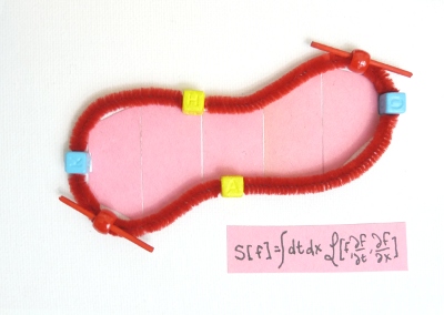
I did not show a slight variation on the function for two reasons. First it would make the graphic much more complicated. Second, a goal of the calculus of variations is to find a symmetry such that when the particular variable is varied, all the derivatives are not changed. The goal is to find a symmetry such that the function does not move.


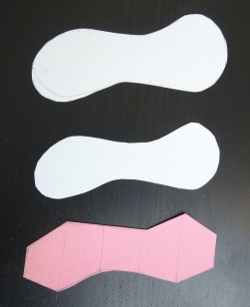Creating these bas reliefs (a fancy way of saying sculptural images) involved iterative  approximations. This was a case of art imitating math.

A three dimensional functional needs a third set of endpoints. The same players take the stage: derivatives as slopes and integrals as areas.

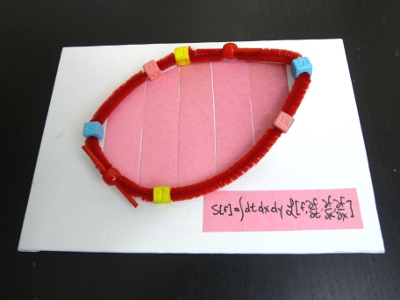
This warped potato chip is a way of representing a 3D functional.

[Corrections: if the function is the pipe cleaner, then as before, this a a 1D parameterization loop in a 3D space. There is one degenerate endpoint. If the function was a volume, then the boundary would be an area. In space-time, the integral could be represented by a volume that persists.]

3D+Time Animations


Continuing on with the theme, a four dimensional functional - can it be done? It cannot be done with a fourth spatial dimension. This is where defenders of work on strings stand up and shout about Kluza-Klein, and how this is so well understood by the bright kids in the class who now have positions at august institutions. 

Using supplies from Michael's Arts and Crafts, I was able to go from a one dimensional functional, to a two dimensional functional, to a three dimensional functional. With all the meandering through their isles, I see no practical way to do four spatial dimensions. Building something helps me believe it.


All representations are flawed in their own ways. If a representation was perfect, then it would be the object in question. In these blogs I have represented things that move and are functions of time by static graphics. This is consistent with the publish or perish tradition of science. Journals and textbooks have long required the static content professors produce.

This is the web. It is sad that I need to use an open format developed over twenty years ago, and at low resolution, but gif89a is good enough. Here is a function wandering around in circles in 3D+time:

[Clarification: The equation and its software uses but one parameter in four places, so this is a 1 parameter curve in a 3D+time space.]

The tx complex plane has a perfect circle. This is a way to represent U(1) symmetry. The ty complex plan has a bow tie. That is the reward for zipping around the circle at twice the speed. The motion in the tz plane is slow. When generating the animation initially, time t went from 0 to 2 pi, and only half of the figure appeared. Once the range was set to run from 0 to 4 pi, the full picture was seen.

The animation repeats. I could call that having periodic boundary conditions. In the classical world, it is simple to create a system that has three different types of rotational symmetry as any Olympic diver will tell you.

There are four pairs of boundaries: . These same characters make up the group E₈, but I think that is just a coincidence. The extremes are reached at different times. The left/right boundary happens at time zero. The edge of near/far along the z axis is reached right at the start. The up/down boundary is touched four times.

It took some programming, but I was able to generate the slopes.

There are four straight lines that wander through the animation. The most motion is seen along the y axis (2t) while the least appears along z (t/2). The thickness of the lines in the ty plane indicates more motion happens there than in the tz plane. At an early point in the animation, I mistook two separate straight lines as one line that was curved. The shadows convinced me that they were really straight lines.

Integrals are possible in animations too. The idea is to draw a line from the origin to every point on the curve. It might take a hundred thousand quaternions in the case, but computers are good at managing that level of detail as this animation shows:


Not quite a Pringle's chip. The superposition of all states shows the curved area one expects to see for an integration. The animations shows how that area is drawn dynamically. The animation is drawn and redrawn due to the periodic boundary conditions.

The function, its derivatives, and its integrals can all be smushed together as happens for functionals:

The smush wipes out the function in yellow in the process, but at least one sees the derivative joining up with the integral in a way similar to static representations.

An animation of a 2D+time function can be created by freezing one of the spatial dimensions:

[Clarification: a 1 parameter curve in a 2D+time space.]

All this motion happens at the same distance from the viewer. This animation is complete when one goes from t=0 to 2 pi.

Take another step down, not allowing any change to appear in the y direction, no up, no down:

[Clarification: a 1 parameter curve in a 1D+time space.]

This animation is a way to represent U(1) symmetry dynamically.

The deepest idea in the pool of the calculus of variations goes by the name "Noether's Theorem".(wikipedia,  Georg von Hippel). A continuous symmetry in an action leads to a conservation law every time. Can we spot both a continuous symmetry and some kind of conserved quantity in this animation? The continuous symmetries are the angles of the circle. One can choose to reside at any arbitrary angle. What is both discrete and conserved? The number of circles is one. No matter what kind of reference frame an observer happens to be in - inertial or non-inertial - there will always be one circle.

The simplest case bothers me. Here only time gets to vary.


Visually this is dead dull. I need a format that could provide an audio track. The drum beat here would not be even. There would be lots of beats at the start and the end, with a slow down in the middle. One could hear that, but not see it unless I did something with how transparent the images are.

The Math

How does the math change going from one to two, three, or four dimensions? Pack all the partial derivatives into one symbol, nabla, the upside down triangle: . The total time derivative in the 1D case becomes this derivative, which has time plus one, two, or three spatial derivatives. The logical flow remains the same. Start with the definition of the action which is a functional:



Why the Omega? The integral is no longer between two endpoints. Now one needs a boundary in however many dimensions are used in the integral.

Consider a small variation in the function f:



The variation is small in the sense that it only depends on first order derivatives of the function f. Because the variations are small, look at the Taylor series for the Lagrangian:



Plug this back into the expression above to cancel out the zeroth order term. The variation with respect to \nabla f can be rewritten using the product rule as the total derivative minus the variation with respect to f like so:



One needs to use Stoke's theorem to work with the middle term. It is a multidimensional analog to the fundamental theorem of calculus. If the boundary is fixed, then the middle term will not make a contribution because the variation will have to be zero on the fixed boundary. For a harmonic boundary condition, the boundary varies, but the variation is the same so again the middle term vanishes. An extremum is achieved if the integrand is zero.



This is the Euler-Lagrange equation for two, three, or four dimensions. At this time, I have no idea how to play with more than four dimensions. Most of this derivation could be made for arbitrary dimensions. I imagine the Stoke's theorem part gets quite tricky for more than 3D+time dimensions.

Speculative, Crazy Animations

In the first blog, I made a mistake with the jargon. Both of these blogs are about the simple stuff, which are called functionals. The hard stuff is relativistic quantum field theory that uses functional integrals to get sums over all possible histories.

The following is techno-visual-speculation on my part. I have had fun playing with quaternion triple products because they look like, but are not an exact match with, the gamma matrices of quantum field theory. They take one path and create 15 others that are related to the original by taking the values of time and space and shuffling them completely. I couldn't resist taking my 3D+time function and seeing what the quaternion triple products would do to it.



…(all 16 possible triple products)

Too much is happening for me to "get it". I decided to try and look at the integral form, where every point connects back to the origin. My Linux box did not like the idea. It choked on the 1.6 million quaternions I fed it with my user-hostile software. I was able to grab the animation part, which looks like this:

This starts and ends as a Mr. Octopus of Spiderman fame. Dead in the middle, every point gets in line. I didn't expect to see that. Time to slow down the skis, but this was a fun run for me :-)

Doug

Snarky puzzle: Lots of theory, little practice. I will steal a problem from David:

Given a fixed length, closed boundary (like a fence), what shape boundary will maximize the enclosed area?

Next Monday/Tuesday: Snark Attack Avoided with Answers