

Earlier this week I argued that biological systems posses dynamical properties that are biologically important, and understandable primarily through mathematical modeling. As an example, I discussed a paper that explored the advantages of double positive feedback loops in bistable switches.
I glossed over the math behind the model because of space and time constraints. (Constraints on a blog, you wonder? Well, I ran out of time, and once a blog post gets beyond 1000 words, the number people who read it to completion probably drops exponentially for every word over 1000.)
However, the math is one of the most interesting parts, and without it, my argument for the need to model may seem less persuasive. So let's delve into the model a little.
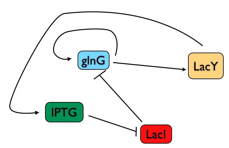
First, a review of the the E. coli genetic switch built by Chang, et al. In my crude drawing below (genes and their cognate proteins are merged into single elements in my drawing), note that:
1) The output of the system is LacY - when the switch is on, LacY is produced; when it's off, LacY is not made.
2) The controllable input is the chemical IPTG - the scientists add a given concentration of IPTG to the bacterial growth and then determine whether LacY is produced or not (i.e., is the switch on or off).
3) The production of LacY is ultimately controlled by a direct transcriptional activator, GlnG. So as we analyze this system, what we're really interested in is the steady state level of GlnG - because the entire circuit is only in a stable state when the concentration of GlnG is not changing.
The steady state concentration of GlnG is easy to define: when the production and degradation rates of GlnG cancel each other out, when they are equal.
You can show this graphically in what is called a rate-balance plot:
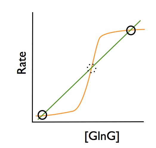
This graph represents the production and degradation rates of GlnG at a single, unchanging concentration of IPTG. The y axis shows the rate of production or degradation, and the x axis shows the concentration of GlnG. Since the degradation rate of GlnG is simply a rate constant a times the concentration of GlnG (deg. rate = a*[GlnG]), degradation rate is a simply linear function of GlnG concentration - the straight diagonal line in the graph.
The production rate of GlnG is more complex. As you can see in the circuit diagram, GlnG feeds back on itself to stimulate its own production (the first positive feedback loop). The dependence of the production rate on GlnG concentration is more complex, resulting in the sigmoidal curve. (One way to model this would be to model the dependence with a Hill function, right out of Biochemistry 101).
So where are the steady state points? Exactly where the two plots intersect - where production rate equals degradation rate. Those points are circled in the graph - the two stable states of low and high levels of GlnG, which result in low or high levels of LacY. (The dotted circle is an unstable steady state.)
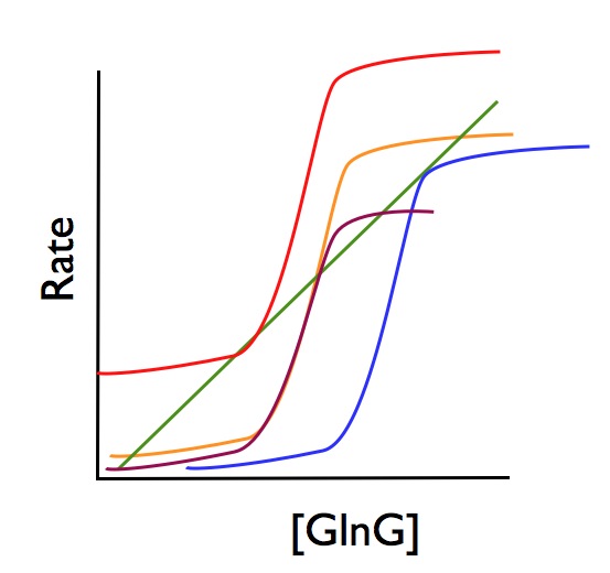
This basic setup is true whether you have one positive feedback loop or two. As the authors write, "Factors controlling the shape of the S-shaped activator production curve, such as the steepness of the curve or its absolute height, control the range of bistability of the system." In other words, as you manipulate elements of the system, like the number of feedback loops or the values of the parameters, you change the distance between the two GlnG steady state points.
So, as you can see in the following figure, you can change where the production and degradation curves intersect, by either shifting the S-curve (by changing the IPTG concentration), or deforming it (by changing the wiring of the circuit.)
The math behind these models is fairly simple. The degradation rate is just:
deg. rate= k*[GlnG]
k here is a rate constant.
The production rate is also fairly simple. In this particular paper, the authors didn't include the specific form of the function they used, but you can use a Hill function to model the binding of a transcriptional activator to a promoter. So, if we want to model the rate of production of GlnG as a function of GlnG (see the wiring diagram above), you can write:
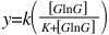
Here, y is the synthesis rate, and k is a rate constant. You can add terms to this equation to include the effects of other regulators on the synthesis of GlnG, like LacI.
These equations are in fact differential equations - the rate in this case being dGlnG/dt. But that doesn't matter when it comes to drawing rate balance plots - you're not solving these equations, you're just drawing the rate as a function of the concentration of a component.
This is an extremely brief overview, but the graphical approach makes it easy to see what's going with bistable switches. To learn more, check out this paper (PDF) by one of the leading researchers in this area, Stanford's James Ferrell.
Read the feed:


Comments