The presentation of data is a very rich subject, on which there is a whole lot to discuss, even by restricting to the issues relevant to our dear field of experimental high-energy physics. Usually too little thought is given to it, even by expert researchers, so I thought that maybe today I would offer here some ideas on one very basic issue, the one of how to choose the width of the bins of a histogram.

You all know what a histogram is: a set of bars whose height is proportional to some quantity one wishes to display, lined up along an axis which represents a parameter. For discrete parameters the bars usually may divide the data into well-distinguishable subsets -say when the parameter is a country and the height of the bars represents their GNP. But for continuous parameters, the width of the bars affects the information content of the graph significantly.

The choice of bins of a histogram invoves a few general statistical considerations, which depend on the use that is made of the distribution. One should first of all distinguish from the outset the use of binning for pure display purpose and the binning of the data as a pre-processing tool. Note that the distinction is clear in particle physics, but less so in other fields of research, when the concept of image processing somehow blurs the boundary.

A) When the data are binned before they are collectively input to a statistical method aimed at extracting an estimate of a parameter of interest (such that the method receives as data input the bin contents only), one should be aware that such pre-processing unavoidably involves a loss of information. Of course: you lose track of the exact value of the parameter for a given event, in exchange for a range -the one spanned by the bin where the event falls.  In this case, one should note that the loss may or may not be critical to the measurement, and it may be an acceptable price to pay in exchange for a large decrease of computation time in complex problems.    

B) Different is the case when the data are divided into subsets depending on the range taken by an observable, and each subset is then analyzed separately. The loss of information due to the binning of data is then irrelevant or absent (e.g. if the observable is ancillary to the measurement being performed, or if the different subsets are independent), and the focus is on other considerations, such as the desire to ease the comparison or combination of results with earlier ones (in which case it may be advantageous to reproduce the pre-existing bin ranges), or the need to control the statistical uncertainty of the measurement across the bins.

C) In general, in order to extract information from the distribution of an observable quantity it is recommendable the use of unbinned techniques, the most classic example in HEP being unbinned likelihood fitting. In that case, the issue of bin size to display a distribution becomes essentially a cosmetic one. Even then, a few simple recommendations can be given.

1. For display purposes, the bin size should be preferably smaller than the experimental resolution of the quantity being drawn. Wider bins hide too much information from the user, and they further bring in a dependence of the perceived location of a feature of the distribution on the location of the bin edge.
2. The only concern with too narrow bins is instead that random fluctuations might distract the user's attention from the important features of the distribution. In the prototypical case of the histogram of the reconstructed invariant mass of a decay system in the presence of significant background and/or when the signal strength is just above detectability, a bin size smaller than the expected RMS of the particle signal should be chosen (when by "RMS of the particle signal" is understood that one should consider the detector resolution convoluted with the particle's natural width). A sound choice is to have the signal distribute into at least five adjoining bins. 
3. Even in the case of the prototype problem given above, one may consider the option of avoiding the binning altogether, and rather produce a cumulative distribution of the invariant mass, with tick marks at the location of each event. Such a method however is impractical for large sample sizes.

Let us see how the criteria above score for three typical experimental cases.

Case one: significant bump, small statistics. Four possible choices with W=0.25*RMS, 0.5*RMS, 1.*RMS, 2.*RMS.

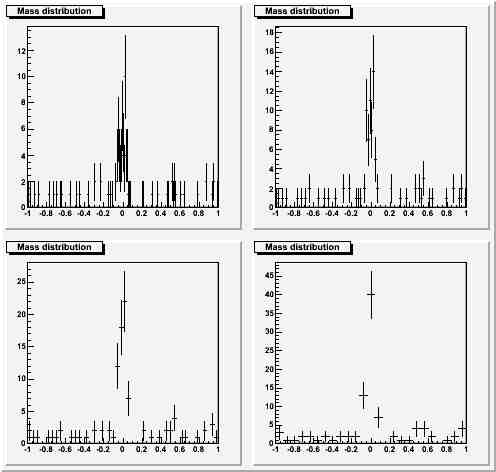Here you can see that a narrow binning does not spoil the view, while the widest binning hides significant information (on the signal width itself).

Significant bump, large statistics, same choices for the bin width as above:


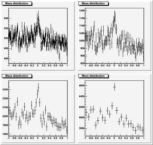
I think any discerning physicist would choose one of the narrowest choices for the bin size in this case. Already a bin size equal to the RMS (lower left panel) is probably hiding too much information.

Barely significant bump, small statistics, same choices of binning:


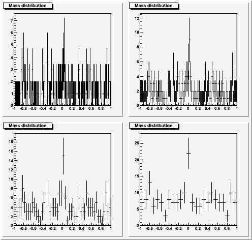
Here I believe the narrowest binning is a bit extreme, but again I am inclined to believe that the wider ones do a poor service: the "fit by eye" does evidence a fluke at zero in the widest bin case, but there is no support from the adjoining bins in the hypothesis that the fluke comes from a real signal. In this case the binning equal to half the RMS (top right) appears optimal to me.


I would be happy to hear your comments or opinions on the matter...