When physicists working in a collaboration want to publish the observation of a new effect in the data, they need to first convince their peer that what they are observing is real, and not the product of a weird fluctuation.

Statistical fluctuations are everywhere, and they sometimes do produce weird results. We are only human, and when facing unlikely fluctuations we are invariably tempted to interpret them as the manifestation of something new and unknown.

Because our weakness is well understood not only by psychologists but also by men of Science  ;-) , there are remedies, though. Physicists who understand statistics (there are a few) have cooked up a very simple recipe, for instance, to decide when somebody has the right to claim the observation of a new phenomenon: it needs to equate to a 5-standard-deviations or larger effect.

A five-standard deviation effect (also known as "five-sigma") is a very, very unlikely occurrence: it corresponds to a probability of 270 times in a billion. Smaller than the probability of throwing a natural seven eight times in a row. Smaller than the probability of picking a number at the roulette and winning four times in a row. It never happened to you, did it ? Five sigma is comparable to the chance of reaching the end of a working day without spam in your inbox. Five sigma corresponds to the probability that a randomly chosen human being reads this blog. Yes, that small.

The problem with the above stipulation ("observation can be claimed for a new particle only if the evidence amounts to a 5-sigma or larger effect") is that it is all too easy to set up a computation of the probability of what you observe and come up with a wrong number. It is so easy that if you are a researcher and your ethical standards are less than iron-clad, you can easily tweak your computation to inflate the result of your estimate, "demonstrating" that what a rigorous calculation would estimate as a 4-sigma fluctuation is in fact a 5-sigma or larger effect.

There are two reasons why the risk of an overestimate of significance is real and present in experimental physics. The first is that significance is not a physical quantity, so a researcher will not be motivated to make his or her best to estimate it with the utmost possible accuracy -it suffices to just showing that it is large enough for the "evidence" (3-sigma, a 0.2% or smaller probability) or "observation" claim (5-sigma) to be well-grounded. The second is that statistical significance is not even well-defined. There is a degree of arbitrariness in its definition, in fact.

A simple example

Imagine you inspect a 50-bin histogram displaying the reconstructed mass of a system of particles, in events collected by your detector. This quantity is expected to be evenly distributed in the bins of the histogram, such that you expect 100 entries in each bin, on average. However, you notice that while 49 bins have all about 100 entries (say, anywhere from 85 to 115: the typical scale of the statistical fluctuations of 100 is +-10 or so), one bin is surprisingly high, containing 140 entries. Since you expected only 100 entries in that bin, just as in the others, you start thinking that the excess might be due to the production of a new particle. This unknown new body would decay into the system of particles you selected in each event, enhancing the number of entries of the bin corresponding to its physical mass.

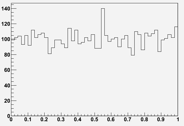You get excited, since you know that the "standard deviation" of the entries in each bin is the square root of the entries. If all bins have on average 100 entries, that was your prediction for the high bin, too: and since the square root of 100 is 10, you are observing an excess of 40+-10 events in that bin! A four-sigma excess ?

Indeed, the chance that 100 counts fluctuate to 140 or more is about one in 25 thousand. The problem, however, is that you had not predicted beforehand which bin would contain the signal. A fluctuation is just as likely to occur in each of the bins, and there are 50 of them. So you are looking at a 0.2% effect, not a one-in-25-thousand one! There is therefore no sufficient ground to claim for "evidence" of a new particle.

The above is an example of the so-called "look-elsewhere effect": the estimated probability of a unlikely effect must be multiplied by the number of ways that the effect could have manifested itself. You had the freedom to "look elsewhere" before picking that bin as your candidate signal, so the probability needs to account for that.

Getting technical

I discussed in more detail and with real-life examples the look-elsewhere effect elsewhere, in a rather popular post. After having introduced the issue with the example above, here I would like to discuss a rather technical question that may arise when one sets up a calculation of the probability of an observed fluctuation. The set up attempts to include the look-elsewhere effect, but fails in a subtle way.

Imagine you are looking again at a mass histogram such as the one described above, and again you see an excess in a part of the spectrum. This time, rather than just counting the entries o f a single bin, you do what physicists do in these cases: you fit the fluctuation as a Gaussian signal on top of the flat background.

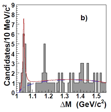Note, incidentally, that I am simplifying matters here to some extent. A particle mass reconstructed by your detector will not, in general, yield a Gaussian signal. It will in general be the convolution of the Breit-Wigner lineshape of the particle with a Gaussian smearing representing the experimental resolution on the measured quantities with which the mass is computed. Also, the "combinatorial background" might not be flat (in fact it is not, in the example figure shown on the right). However these details need not concern us here, since they do not affect the conclusions we will draw.

So you fit the fluctuation and obtain a nice interpretation of your data: it seems that on top of a "combinatorial background" (a term that characterizes the mass values of the histogram as random combinations of particles not produced all together in the decay of a more massive body, thus distributing with equal probability in the histogrammed mass range) there is a decay signal of a new particle. A mass bump.

On statistical grounds, the most accurate measure of the strength of the signal is arguably the so-called "delta log-likelihood" of two fits to the data: the one including the Gaussian signal (what is called the "alternate hypothesis", which assumes there is a new signal in the data), and one performed by pretending that the data follow a flat distribution (the so-called "null hypothesis"). The Delta-log-likelihood is a property of the pair of fits taken together. The larger the delta-log-likelihood, the better is the alternate hypothesis than the null.

I will not provide here the recipe to compute the delta-log-likelihood by the way, because it is straightforward if you are an insider, and complicated if you are not. Suffices to say that it is a function of how well the alternate model passes through your data points, and how badly the null model does. So let me continue.

To quantify what the Delta-log-likelihood you found really means -i.e. how justified is the alternate hypothesis- you might take a shortcut using some formulas that translate it directly into a probability; however this is dangerous in some cases. Much better is to proceed to construct toy pseudo-experiments. A toy pseudo-experiment is a set of data different from the one you actually obtained in the real experiment, but one you could have obtained, if the data distribute according to a model you pre-define; in this case, a flat mass distribution, containing no signal. You had N entries in the data histogram, so you construct a pseudo-histogram by randomly picking N mass values in the studied range. "Random" here means that the mass you pick for each event has a flat probability distribution: you are generating a pseudo-dataset following the null hypothesis.

Then you fit with the two different hypotheses, and come up with a Delta-log-likelihood. This will in general be smaller than the one you observed in the real data, of course: the pseudo-histogram will usually not show very unlikely fluctuations such as the one which motivated your study in the first place.

By repeating the pseudo-histogram generation and fitting a large number of times -say a few million times-, you may come up with a smooth distribution of Delta-log-likelihood values. Most of your pseudo-histograms will return small values, but some will occasionally show a large signal somewhere in the spectrum, and the fit will like to pass a Gaussian through those data points, getting a large difference of log-likelihood with respect to the fit to the null hypothesis.

You may now compare the result you obtained in real data (the red line in the figure above) with the ones in the distribution of Delta-log-likelihoods obtained from pseudoexperiments: counting the number of pseudo-histograms with a Delta-log-likelihood equal or larger than what you see in real data, and dividing by "a few millions" (the number of generated pseudo-histograms), will produce a veritable estimate of the probability that your real data distributes according to the null hypothesis. It is the number you were looking for, and it accounts for the look-elsewhere effect, since you allowed the fits to pick a signal irrespective of its location in the pseudo-histograms.

Enter the other parameter - the width

So far so good -although we are already hiding some subtle details here. Whatever fitting machinery you are using, you need to verify that it is capable to pick the largest fluctuation in the whole spectrum: this is required because fits are usually lazy, and if they get stuck in a local minimum they will fail to make the best possible use of the degrees of freedom allowed by the alternate hypothesis (the Gaussian signal, whose mass is a free parameter in the fit).

But let us suppose that indeed, the minimization routine performs a fine scan of the mass values attributable to the Gaussian signal, and thus indeed reports for each pseudo-histogram the largest fluctuation, so that a correct Delta-log-likelihood is obtained.

This far we have neglected to mention that a Gaussian has not just a mean value (the mass of the tentative new signal) and a height (which the fitter tries to adapt to the high bins): the Gaussian has also a "sigma" parameter which describes its width. And here we come to the point I want to discuss in this article, ultimately.

The experimenter might see a narrow bump in the data, and decide that he will check with pseudoexperiments how likely it is that such a narrow bump is seen. But the width, just like the mass, was not known beforehand -the experimenter was not looking explicitly for a narrow state when he first produced the histogram, ending up reckoning with the bump-like excess. So he needs to vary the width as well in the pseudohistogram fitting.

Or does he ?

It so happens that fluctuations that resemble large-width Gaussians less frequently produce extreme values of the Delta-Log-Likelihood between alternate and null hypotheses than fluctuations resembling narrow-width ones. This is due to the fact that a larger width signal is better approximated by a flat distribution than a narrow width one. Or, if you want, it is due to the fact that a large-width signal will produce smaller variates with respect to the null hypothesis, albeit in a wider range. This feature is more evident in small-statistics histograms, where one constrains the number of events observed in the data (N) and produces pseudo-histograms with N events when calculating the Delta-log-likelihood distribution.

Please note that the above problems depend on the specific details of the histogram (number of bins, entries, etcetera). So it is hard to draw general conclusions. However one might speak of an "inverse look-elsewhere effect" in some cases: by making the signal search "more general"
(i.e., allowing for larger width signals), the experimenter may end up evaluating a significance that is smaller than what it should be: quite the opposite of the normal look-elsewhere effect!

An open issue

So what happens to experimenters confronted with the problem of correctly evaluating the significance of a narrow bump ? Should they fix the width of the Gaussian they uses in their "alternate fits" to the pseudoexperiments ? Or should they allow for the minimization routine to freely vary the width parameter as well ? And if so, how should the returned distribution of Delta-log-likelihood be interpreted ?

Strange as it may seem, these questions do not have an agreed-upon, standard answer. This, in my opinion, is bad for experimental physics, since experimenters are often left alone in cooking up a recipe for the evaluation of the statistical significance of their signals. It ultimately is the reason why when a speaker representing his or her collaboration presents at a conference the tentative observation of a new particle or effect, all the other physicists will take it at first with a sceptical attitude.

The devil is in the details of the computation of the significance, and those details are usually not accessible -another problem of today's organization of research in experimental physics! Take the DZERO observation of the Omega B baryon in 2008: as I wrote in a series of posts, I did not believe that they had estimated the significance of their signal correctly, since my own calculation turned out to produce a smaller result. I posted a few articles online and even published a preprint on the matter, but I received no direct reply.

Oh well... DZERO is not alone. The CDF collaboration published in 2009 the evidence of a meson called Y(4140) and quoted a significance based on pseudoexperiments which varied the width in a large interval. I will discuss the case of the Y(4140) in more detail in a future post, after CDF will publish an update of that analysis based on a larger data sample: they are now finding a larger than 5-sigma significance...